|
|
|
Copyright © 2004 by the author(s). Published here under license by The Resilience Alliance.
Go to the pdf version of this article.
The following is the established format for referencing this article:
Carpenter, S. R. and W. A. Brock. 2004. Spatial complexity, resilience and policy diversity: fishing on lake-rich landscapes. Ecology and Society 9(1): 8. [online] URL: http://www.ecologyandsociety.org/vol9/iss1/art8/
A version of this article in which text, figures, tables, and appendices are separate files may be found by following this link.
Report Spatial Complexity, Resilience, and Policy Diversity: Fishing on Lake-rich Landscapes Stephen R. Carpenter and William A. Brock
University of Wisconsin-Madison
- Abstract
- Introduction
- A Lake District Model
- Theory for a Single Lake
- Theory for Multiple Lakes
- Discussion
- Responses to this Article
- Acknowledgments
- Literature Cited
The dynamics of and policies governing spatially coupled social-ecological mosaics are considered for the case of fisheries in a lake district. A microeconomic model of households addresses agent decisions at three hierarchic levels: (1) selection of the lake district from among a larger set of alternative places to live or visit, (2) selection of a base location within the lake district, and (3) selection of a portfolio of ecosystem services to use. Ecosystem services are represented by dynamics of fish production subject to multiple stable domains and trophic cascades. Policy calculations show that optimal policies will be highly heterogeneous in space and fluid in time. The diversity of possible outcomes is illustrated by simulations for a hypothetical lake district based loosely on the Northern Highlands of the State of Wisconsin. Lake districts are frequently managed as if lakes were independent, similar, endogenously regulating systems. Our findings contradict that view. One-size-fits-all (OSFA) policies erode ecological and social resilience. If regulations are too stringent, social resilience declines because of the potential rewards of overharvesting. If regulations are too lax, ecological resilience is diminished by overharvesting in some lakes. In either case, local collapses of fish populations evoke spatial shifts of angling effort that can lead to serial collapses in neighboring fisheries and degraded fisheries in most or all of the lakes. Under OSFA management, the natural resources of the entire landscape become more vulnerable to transformation because of changes in, e.g., human population, the demand for resources, or fish harvesting technology. Multiplicity of management regimes can increase the ecological resilience, social resilience, and inclusive value of a spatially heterogeneous social-ecological system. Because of the complex interactions of mobile people and multistable ecosystems, management regimes must also be flexible over time. A rights-based scheme may facilitate policy regimes with appropriate spatial patterns and intertemporal fluidity. In lake fisheries, habitat protection adds an important dimension to policy design. Habitat is a slowly changing variable that creates ecological resilience and thereby provides managers with a broader range of options.
KEY WORDS: angler dynamics, fish habitat, inclusive value, lake, lake management, landscape ecology, multiple attractors, natural resource policy, resilience, social-ecological system, spatial dynamics, sport fishery, sport fishery, sport fishery management.
Published: March 15, 2004
Waves of change may break over landscapes following exploitation by humans. Significant ecological changes have followed human occupation of new islands or continents (Redman 1999, Flannery 2002). Some ancient civilizations underwent booming growth followed by declines associated with environmental degradation (Redman 1999). Modern parallels are found in the patterns of urban sprawl, land development, and loss of natural resources called "leapfrog degradation" by Likens (1992). The generic problem of large-scale resource transformation has some common elements: multiple regimes of ecosystem dynamics, landscapes of diverse ecosystems, spatial connections by flows of water, chemicals, organisms and people, and human actions. These elements may be combined in diverse and complex ways. It seems likely that these phenomena could be better understood through modeling studies, but relatively few models have combined social-ecological dynamics with processes at multiple spatial and time scales.
Ecological, economic, and social theory can provide many useful elements for the construction of appropriate models. Ecosystems on heterogeneous landscapes are connected by flows of organic energy, water, chemicals, and organisms (Turner et al. 2001). Ecologists have found that ecosystems can be understood by focusing on interactions at a few key scales of space and time (Levin 1999). Certain residence times and certain spatial extents have overarching importance in the dynamics of a given landscape. Such insights provide the rationale needed to suppress superfluous detail and formulate useful models for understanding.
Economic theorists have addressed the management of large numbers of heterogeneous, modular organizations connected by mobile populations of rational actors. Standard economic theory shows that, if enough of certain conditions are met, the private interests of many diverse actors can be aligned to the social interest through the appropriate design of incentives. For example, competitive equilibria under decentralized markets are Pareto optimal if certain conditions are met, i.e., it is not possible to reallocate resources from the equilibrium allocation to make one agent better off without making some other agent worse off. Standard textbooks such as Varian (1992) address the relationship between competitive equilibria and notions of optimal allocations. Mas-Collel et al. (1995) give general methods of designing incentive schemes to align the private interests of individual decentralized agents to achieve social goals.
Several modeling studies have combined ecological and economic principles to study the behavior of spatially heterogeneous ecological-economic systems (Bockstael 1996, Brown and Roughgarden 1997). Spatial models of commercial fisheries were introduced by Hilborn and Walters (1987) and Allen and McGlade (1987). More recently, spatial models of commercial fisheries have been used to study the interactions of dispersal by both the fish and fishers (Sanchirico and Wilen 1999, 2001). This work shows the possibility of "spatial cascades" of fishery impacts across patchy environments. Our paper adds to this literature by considering three scales of change in the spatial dynamics of fishers and a richer ecosystem model that includes habitat effects, depensation, and trophic cascades. An important feature of our study is the insularity of lake fisheries. Spatial models of marine fisheries address movements of both fishes and fishers. In lake fisheries, the individual lakes are connected by fisher movement. Lack of immigration increases the vulnerability of lake fisheries to depensatory collapse, as represented in our model.
Social theorists have considered the conditions necessary for the establishment of long-lasting systems for the management of common property resources, including complex ecosystems (Ostrom 1990, Ostrom et al. 2002). Economists have studied the same kinds of problems and their consequences for overall social welfare. In the contentious context of international trade and globalization, for example, several authors (Chichilnisky 1994, Brander and Taylor 1997, B. Copeland and M. Taylor, unpublished manuscript) consider modifications in the standard welfare theorems of international trade caused by the presence of commons and other problems related to incomplete property rights.
A major cause of economic welfare loss stemming from commons-related problems is the dilution of property rights that results from open access to natural resources such as fisheries. These problems require modification of the basic welfare theorems of competitive analysis in economics. Social science research in this area focuses on topics such as:
- improving the clarity and transferability of property rights (Repetto 2001);
- locating sufficient conditions for the existence of transparent monitoring systems that are credible to all agents and enforceable at reasonable cost (Ostrom 1990, Ostrom et al. 2002);
- describing conditions favorable to the endogenous emergence of self-enforcing agreements and other mechanisms of controlled access without assistance from government (Ostrom 1990, Ostrom et al. 2002);
- determining the conditions under which government intervention can achieve workable efficiency of the managment of particular natural resources in, for example, fisheries (Repetto 2001);
- studying the mechanisms for collective choice and conflict resolution (e.g., Axelrod 1997);
- identifying the conditions that favor the construction of economic mechanisms such as surrogate markets, tradeable rights, amenity bundling, securitization, and other devices to help ameliorate the problem (Chichilnisky and Heal 1993); and
- describing and implementing generally desirable attributes of environmental management institutions, whether self-organized or catalyzed by an appropriate unit of government.
Sport fish management, the specific focus of our article, has assimilated some but not all of these insights from social science (Mather et al. 1995, Radomski et al. 2001). Nevertheless, the management of sport fisheries illustrates all of the above problems and concepts very well. In particular, the focus (B. Copeland and M. Taylor, unpublished manuscript) on the interaction between the size of a natural resource stock such as fish, the temptation to cheat faced by each fisher, and the probability of getting caught, which, in turn depends on resources devoted to enforcement, is germane to our work.
Despite the achievements of the separate theories, the dynamics of even simplified ecosystems on spatial mosaics pose significant challenges for optimal management of renewable resources. Even in spatially homogeneous systems, the stochasticity, time lags, and multiple stability domains of ecosystems create significant difficulties (Walters 1986, Carpenter 2003, Ludwig et al. 2003). In part, these difficulties arise from the different domains of the theories and the lack of integration among them (Gunderson and Holling 2002). Although panarchy theory does integrate these domains, it is a paradigm, not a specific model of a particular social-ecological system (Gunderson and Holling 2002). Additional assumptions leading to system-specific models framed in terms of observable quantities are necessary to evaluate general ideas relevant to the dynamics of social-ecological systems.
Natural processes such as hydrologic transport or animal migrations have long been known to link ecosystems on landscapes. There is growing recognition that the high mobility of humans is a significant factor in ecosystem change. This paper addresses the dynamics of heterogeneous ecosystems linked primarily by the activities of people who can move rapidly among the individual ecosystems. Such situations occur in forestry, some forms of agriculture, hunting, fishing, and ecotourism. At a general level, we wish to understand the patterns that emerge from unregulated human use of heterogeneous landscapes and the policies that might shift the outcomes toward particular goals. As a specific example, we consider the fisheries of a lake district in which many individual lake fisheries are linked by the activity of mobile anglers. Using a coupled, spatially specific model of the social-ecological system, we explore patterns of collapse or persistence. Optimal policies turn out to be highly heterogeneous in space and time. We explore the consequences of policies that are simpler and therefore more closely resemble the actual situation in sport fishery management. We find that one-size-fits-all policies lead to lower inclusive value for a lake district and increase the risk of fishery collapse.
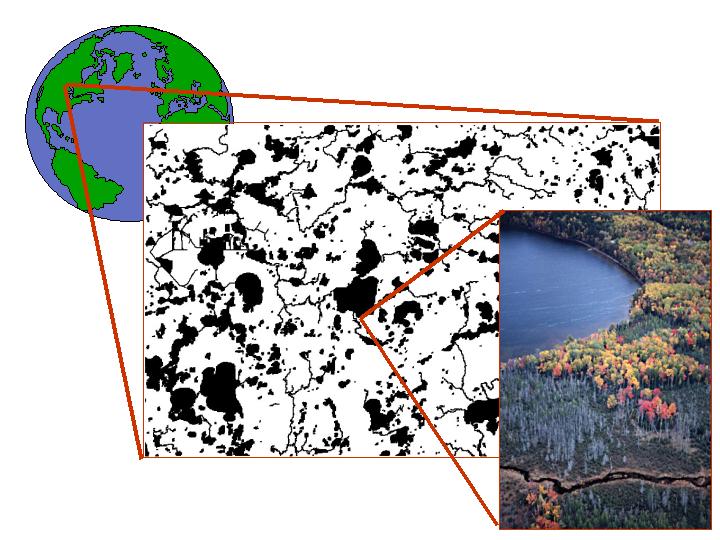
The people who use a particular ecosystem service make choices at several spatial scales. For example, they may choose where to live in relation to the ecosystem service and where in particular to use the ecosystem service. Local exploitation of the ecosystem service may change the ecosystem, thereby affecting future choices by the agents. Landscape pattern may emerge from the interplay of human choice and ecosystem response. The challenge for policy makers is to design instruments that increase the long-term welfare of people throughout the landscape, taking into account spatial dynamics that are potentially unstable. Here, we study this generic problem using the specific setting of a hypothetical lake district. Lakes, like other ecosystems, are not homogeneously distributed across the planet. They tend to be concentrated in certain regions known as lake districts. Lake districts, because of their abundant aquatic resources, are often the foci of human activities such as agriculture, forestry, fishing, hunting, and ecotourism. For a detailed description of the social-ecological system of a particular lake district, see Peterson et al. (2003a).
The socioeconomic system of a lake district can be represented at three scales (Fig. 1). The first scale is that of the individual angler deciding how much time to allocate to angling vs. other activities. This part combines ideas from the standard microeconomic theory of the household (Becker 1991) and studies of angler behavior (Hudgins and Davies 1984, Noble and Jones 1993, Hunt and Ditton 1997, Cox and Walters 2002a, Beard et al. 2003a). The second scale is the choice of location within a lake district, i.e., the choice of which resort to visit or which lakeside cottage to buy. We refer to this location as the base lake. The third scale is the choice to visit or live in the particular lake district vs. living or spending vacation time in a different place.
|
Fig. 1. Three spatial scales of decision making by agents in the model. From a global set of possibilities, agents choose a lake district. Within the lake district, they choose a base lake on which to purchase or rent a cottage. From the cottage, they allocate time to activities that may include fishing on their home (base) lake or fishing on another lake. The diagram depicts part of the Northern Highland Lake District, Wisconsin, USA (Peterson et al. 2003).
|
We associate these spatial scales of decision making with particular time scales by adjusting the rate constants for implementing the decisions. We assume that the decision to visit or live in the lake district is relatively slow, i.e., migration into or out of the lake district occurs at a slower rate than the other decisions. In contrast, decisions about which lake to fish change rapidly, representing the hour-to-hour or day-to-day decision making of mobile anglers. The choice of base lake is assumed to occur at an intermediate rate. Anglers can change base lake less often than they change their fishing site, but will relocate within the lake district more readily than they will move to a different region altogether. Obviously not all the lakes in the lake district are equally accessible to people or equidistant from major highways and population centers.
We focus on the ecosystem service of sport fishing. Sport fisheries are affected by human action in numerous ways, including direct effects of harvest (Cox and Walters 2002, Post et al. 2002, Beard et al. 2003a) and the indirect effects of modifying habitat (Christensen et al. 1996, Olson et al. 1998, Schindler et al. 2000). As a result of these activities, sport fish populations can be altered significantly (Mosindy et al. 1987, Cox and Walters 2002, Post et al. 2002, Beard et al. 2003a). The status of some sport fisheries has been referred to as an "invisible collapse" (Post et al. 2002).
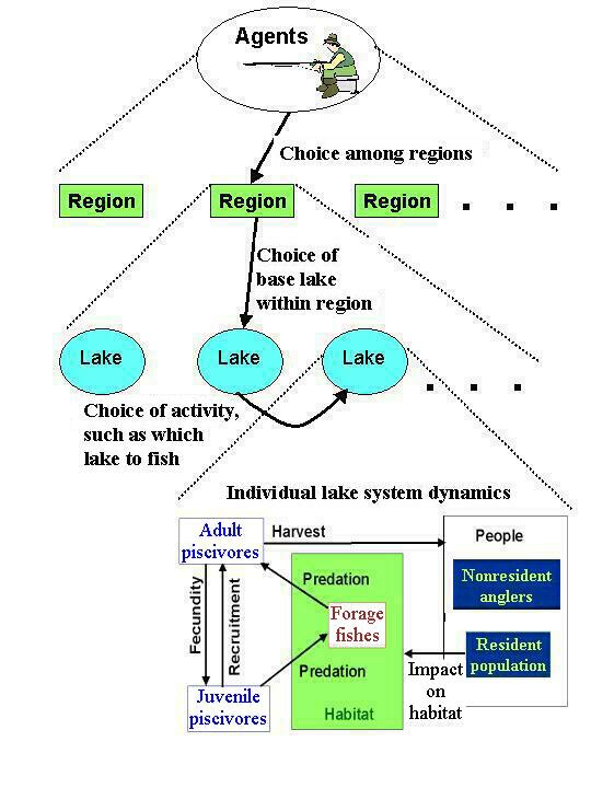
The model (Fig. 2) considers a large population of people who make a series of choices related to fishing. They choose which of many regions to live in or visit. One of these regions is the lake district that is the focus of the model. The model addresses the dynamics of people within this focal lake district. Within the district, each person chooses a base lake or lake on which the person resides while in the lake district. At his or her base lake, the individual angler chooses from a portfolio of activities that include nonfishing activities as well as fishing on various lakes. The lakes are connected by the anglers and differ only in the number of anglers present at any given time. Resident anglers both harvest fish and affect the shoreline habitat, whereas visiting anglers only harvest fish. The food web model is a trophic triangle (Ursin 1982). The game fish population preys on forage fishes as well as other prey, and the forage fishes eat juvenile game fishes. The refuge for predation for juvenile game fish and their vulnerability to consumption by forage fishes depend on the shoreline habitat.
|
Fig. 2. Schematic diagram of the social-ecological system model.
|
In this paper, ecosystem dynamics are deterministic. We assume that anglers and managers know the true model for the underlying ecosystem dynamics and measure ecosystem properties without observation error. Clearly, these assumptions are unrealistic. Ecosystems are stochastic, ecological data contain substantial observation errors, and human agents have imperfect information and behave in boundedly rational ways. Nevertheless, the deterministic, perfect-information case is a valuable benchmark for understanding the potential dynamics of the system. We show that certain kinds of complexity emerge from this simplified situation. Even greater surprises are likely to emerge when realistic learning dynamics and boundedly rational behaviors are introduced into the model. Other work has exposed some of the patterns that emerge when uncertainty, learning, and bounded rationality are considered in the management of a single lake or fish population (Ludwig 1995, Walters 1986, Carpenter et al. 1999, Janssen and Carpenter 1999, Carpenter 2003, Peterson et al. 2003b). In the spatially heterogeneous setting described here, new complexities are likely to arise (Allen and McGlade 1987, Sanchirico and Wilen 1999, 2001). We leave these as a topic for further research.
The single-lake case is a useful starting point. It introduces the model for short-term decision making by anglers, the simplified lake ecosystem model, and the approach to policy analysis that will be used throughout the paper. In the single-lake case, it is easy to grasp the factors that affect the stability and resilience of the fish population. Habitat modifications interact with angling effort to determine the resilience of the fish population and, ultimately, the long-term utility of the fish stock for the anglers.
In this section of the paper, we first introduce a simple model for the allocation of fishing effort by anglers. The lake ecosystem model is then explained. An approach for calculating policies that maximize yield under certain steady-state assumptions is presented and analyzed. Indices of ecological and social resilience are considered. Finally, we discuss the relationship of the single-lake results to some related work on management of lakes and marine fisheries.
Angler choiceConsider the problem of a representative angler who will decide how much time, τ, to allocate to fishing. All symbol definitions are collected in Appendix 1. The utility for the angler is
 | (1) |
where q is catchability, A is fish population size, a is the exponent of a Cobb-Douglas production function (Appendix 2), and S is the shadow price of fishing. In the single-lake case, we use the shadow price to simplify the analysis. In the multilake case, we consider the full range of options available to the angler (Appendix 2), so the shadow price term can be dropped.
Over a period of time short enough that A can be assumed constant, the optimal allocation of time to fishing by a representative person is found by maximizing U over τ. The first-order necessary condition is found by solving dU/dτ = 0 for τ:
 | (2) |
Note that total angling effort by N people will be N τ*. Effort is an increasing function of A, consistent with the findings of Beard et al. (2002) and Cox et al. (2003) for sport fisheries.
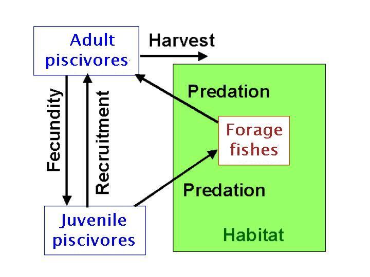
Fish dynamics: a trophic triangleA food web is a network of connections among predator-prey pairs (Paine 1980). In many ecosystems, the existence of a link between two entities depends on their relative body sizes. Size-structured predation is common and important, especially in aquatic systems (Brooks and Dodson 1965). Since the work of Ursin (1982), ecologists have recognized that a basic element of a size-structured food web is a triangle in which the juveniles of a particular species are consumed by larger individuals of another species, which are in turn consumed by the adults of the first species (Fig. 3). For a wide range of situations, such triangles have multiple equilibria (de Roos and Persson 2002). When adults are abundant, the forage fish population is low, juveniles recruit successfully, and the population can reach a positive steady state. This situation has been called "cultivation" (Walters and Kitchell 2001). When the adult population is small because of factors such as heavy fishing or predation by a higher trophic level, the forage fish population is large and may prevent recruitment, causing the fish population to fall to zero. This phenomenon, called "depensation," has a long history in fisheries science (Hilborn and Walters 1992, Walters and Kitchell 2001, de Roos and Persson 2002, Carpenter 2003).
|
Fig. 3. Schematic diagram of the trophic triangle model. Predator-prey interactions in the green box are assumed to depend on habitat conditions.
|
In lakes, habitat structure may influence the predator-prey links of a trophic triangle (Carpenter 2002, 2003). Nearshore or littoral zone habitat is particularly important for small-bodied fishes, including juvenile game fish. Littoral habitat can be altered substantially by human actions such as the clearing of shoreline forest, the removal of fallen trees from lakes, or the introduction and management of higher aquatic plants, with consequences for fish populations (Christensen et al. 1996, Olson et al. 1998, Schindler et al. 2000, Schindler and Scheurell 2002). Our model assumes that predator-prey interactions depend on the condition of littoral habitat (Schindler and Scheurell 2002).
The ecosystem model used in this paper (Fig. 3) is a drastic simplification of lake food-web structure (Cohen et al. 2003). All models are, of course, simplifications that are chosen for particular purposes. We sought a representation of ecosystem dynamics that was simple enough to compute rapidly for large numbers of lakes; addressed an ecosystem service of economic relevance, in this case a fish stock; represented the effects of lakeshore management on the lake ecosystem; and exhibited multiple quasi-stable domains. In addition, the model's dynamics include trophic cascades (Carpenter 2003) that will be useful for future extensions of the model, although this feature is not exploited in the present paper. We believe that the dynamics illustrated by our lake ecosystem models are sufficiently rich to demonstrate important economic-ecological phenomena. Extensions to more complex ecosystem models are left for future research.
A game fish population such as largemouth bass (Micropterus salmoides) or walleye (Stizostedion vitreum) is subject to harvest by anglers (Fig. 3). Adult game fish eat a variety of prey, including forage fishes such as golden shiners (Notemigonus crysoleucas) or rainbow smelt (Osmerus mordax). The forage fishes also feed on diverse prey, but their predation on juvenile game fishes is of particular interest here. Predator-prey interactions depend on habitat structure. As a further simplification, we focus on the effects of habitat on consumption of juvenile game fish by forage fishes. Although the effect of habitat on predation by adult game fish on forage fish could be considered, this added complication does not alter the general findings.
For the purposes of this paper, the model reduces to a difference equation for the dynamics of adult piscivores for the time period between spawning events (Appendix 3). We refer to this time interval as a season. In north temperate lakes, the season generally corresponds to one year. The fishery is open for part of the season. We will assume that juvenile piscivores that survive for one year enter the adult piscivore pool. This assumption about maturation rate is an arbitrary one that leads to useful simplifications. If we assume a longer maturation time, we obtain the same qualitative results, but with additional instabilities because of the time lag of maturation.
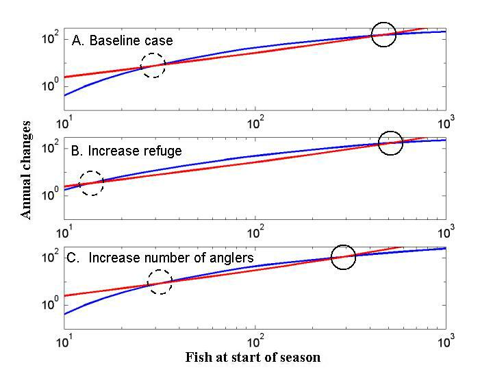
The trophic triangle model has two interesting equilibria (Fig. 4). The right equilibrium point is stable. The left equilibrium point is unstable; small perturbations away from this point either collapse to zero or grow toward the right equilibrium point. The left equilibrium is sometimes called the critical depensation point. The distance between the equilibria is a measure of ecological resilience (Carpenter 2002, 2003).
|
Fig. 4. Rates of overwinter mortality plus harvest (red) and recruitment (blue) vs. the population of adult game fish. Solid circles show stable equilibria. Dashed circles show unstable equilibria (critical depensation points). A represents the baseline case, B the baseline case with a decreased value for the refuging parameter, and C the baseline case with a higher number of anglers. Parameter values are in Appendix 8.
|
A habitat improvement that increases the refuge for juvenile game fishes increases resilience by shifting the unstable equilibrium to the left, so that the population can grow toward the stable point from smaller numbers of adults (Fig. 4B). Conversely, habitat damage that decreases the refuge will decrease resilience by shifting the unstable equilibrium to the right, so that larger numbers of adults are required for the population to grow toward the stable equilibrium.
An increase in angling effort, as might occur when the number of anglers increases and effort per angler stays constant, leads to a decrease in resilience by shifting the stable equilibrium to the left (Fig. 4C). In this situation, a smaller perturbation is required to shift the fish population below the unstable equilibrium. Conversely, a decrease in angler effort, as might be caused by regulation or a decline in the angling population, leads to an increase in resilience by shifting the stable equilibrium to the right. Such a fish population can withstand a larger perturbation without falling below the unstable equilibrium.
Policy for a single lakeIt is useful to consider the case of a single lake before addressing the more complex case of multiple lakes. In both the single-lake and multiple-lake cases, we assume that the ecosystem manager is a rational social planner who attempts to maintain or increase some appropriate measure of social welfare. The welfare for a representative angler at steady state is given by
 | (3) |
In Eq. 3, A(τ)* is the equilibrium fish stock for a specified value of τ. From the manager's perspective, the first-order necessary condition for maximization of expression 3.3 is
 | (4) |
Note that the optimal time allocation from the angler's perspective will usually be different. In calculating her or his optimal time allocation (Appendix 2), the angler accounts only for the direct effect of the fish population on utility. The manager, in contrast, considers the full derivative presented in expression 3.4, which includes the indirect effect of effort on utility caused by the impact of fishing on fish population size.
In practice, the manager's goal can be met by creating incentives or regulations that move the angler's optimal time allocation toward the manager's preference. Appendix 4 explains the calculation of such a policy. Although the theory is straightforward, such policies can be challenging in practice. Repetto (2001) has discussed the practical difficulties of effort regulation in the context of commercial fisheries. To achieve efficiency, economists tend to support the creation of a type of property right, such as an Individual Transferable Quota or ITQ (Hartley 1997, Repetto 2001), in which the Total Allowable Catch (TAC) is set by a central authority in the overall public interest. In the context of a deterministic model where there are no complications because of imperfect monitoring, enforcement costs, or other factors, it may be possible to find a tax to satisfy the manager's goal. Thus, in the context of our simple model, quota setting at a particular level is equivalent to tax setting at an appropriate level.
ITQ systems give fishers incentives to maintain the long-term value of the harvest as well as control over fishing. To make this idea explicit, consider the following scheme. Each citizen could be endowed with a bundle of ITQs, each of which gave her the right to harvest a specified number of fish per year on a particular lake. These ITQs could be traded in an organized market to build packages large enough to support recreational angling for those who care about it. The quota for each lake for each ITQ would be set each year by a professional agency, in public hearings with an open records format that includes invited commentaries from the public. There could be a limit on the number of ITQs that can be owned by any one individual to prevent the concentration of ITQs to a small number of owners (Hartley 1997). Hartley (1997) describes how this system caused the emergence of associations of quota owners who funded projects to promote conservation and quality enhancement in New Zealand. Repetto (2001) describes similar experiences in the Canadian scallop fishery. It seems plausible that the implementation of rights-based schemes such as ITQs could be done in a fair way for sport fisheries. For each particular lake, the management agency would then take over the task of imposing and monitoring compliance with ITQs. In our model, such a scheme has the same effect as the effort tax used as a mathematical device in Appendix 4.
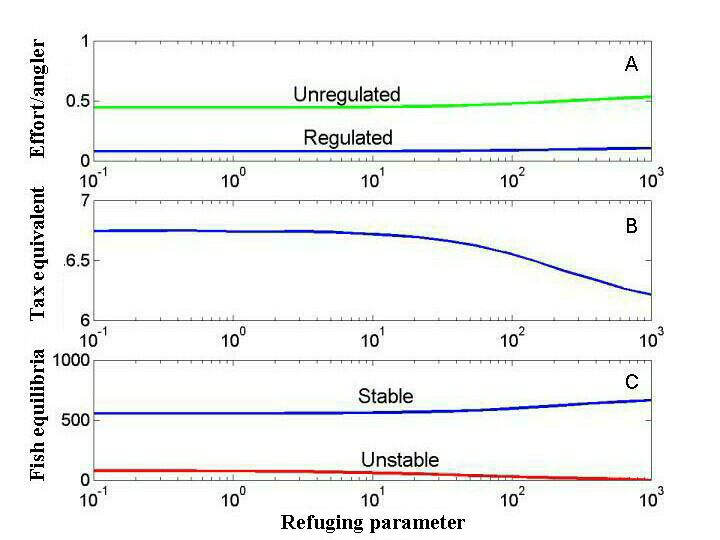
To illustrate the policy calculations for a single lake, fishery variables are plotted against the refuging parameter (h) in Fig. 5. Improvements in shoreline habitat provide more refuge for juvenile game fish and thereby cause h to increase. Unregulated effort per angler is substantially greater than regulated effort per angler (Fig. 5A). Both values increase as habitat improves. The tax-equivalent policy p* necessary to regulate the fishery declines as habitat improves (Fig. 5B). The fish stock at the regulated stable equilibrium increases as habitat improves, whereas the unstable equilibrium point for the regulated fishery decreases as habitat improves (Fig. 5C). Thus, ecological resilience, i.e., the distance between the fish equilibria, increases as habitat improves for the regulated fishery, consistent with intuition from the previous section.
|
Fig. 5. Fishery variables vs. the refuging parameter h. A represents effort per angler with optimal time allocation for the regulated and unregulated situations, B the tax-equivalent policy for the regulated situation, and C the game-fish equilibria for the regulated case. For the unregulated case, there are no positive equilibria for game fish. Parameter values are in Appendix 8.
|
Ecological and social resilience
Resilience is a multidimensional concept (Gunderson and Holling 2002). Many indicators, in many dimensions, are necessary to adequately represent resilience. Here, we present two simple indicators to explore the model and build intuition about the possible dynamics of resilience in the system.
For the relatively simple ecosystem model used here, the calculation of resilience is straightforward (Carpenter 2002). An appropriate index of ecological resilience is
 | (5) |
which is 1 when the critical depensation point Acrit vanishes. RE decreases as A* and Acrit become closer. When the positive stable equilibrium does not exist, we set RE at 0.
Ostrom (1990) discusses many features of social systems that may facilitate, or undermine, successful collective management of common-pool resources. One particular aspect of resilience for the social system is the potential reward for violating fishing regulations. A social regulatory system with a larger temptation to violate regulations may be more fragile, or may require stronger internal norms or more aggressive enforcement, than a social regulatory system with a smaller temptation to violate regulations. Thus, one aspect of social resilience should be smaller if the benefits from violating regulations are greater. An index of this aspect of social resilience is calculated as follows. In general, unregulated time spent fishing, τ*, will be greater than regulated time spent fishing, τ**. An index of social resilience that ranges from 0 (when regulation closes the fishery so τ** = 0) to 1 (when the regulated and unregulated time budgets coincide) is
 | (6) |
In this expression, U is calculated as in Eq. 3. The numerator is the utility obtainable at the equilibrium fish population A(τ**) under the optimal regulated policy τ**, and the denominator is the utility obtainable under the unregulated policy in which unregulated angler preferences τ* drive the fish population to A(τ*).
To illustrate the effects of regulation and ecological variables on resilience, the resilience indicators are plotted against the refuging parameter h (Fig. 6). Social resilience increases as habitat improves (Fig. 6A). Less stringent enforcement mechanisms are required to achieve social objectives when the habitat is better for game fishes. In this case, ecological resilience depends strongly on regulation. In the absence of regulation, ecological resilience is zero, because overharvest drives the fish population below the critical depensation point (Fig. 6B). With regulation, ecological resilience rises as habitat improves, consistent with intuition from the fish population model (Fig. 6C).
Challenges of regulating one lake in a lake districtThe manager's efforts to improve matters in a single lake may lead to perverse outcomes by attracting migrants to that lake from other lakes. This raises the issue of regulation of the whole landscape of lakes. To focus the problem, consider a measure of total welfare for the whole system. Let there be N people in the whole system. Let Wu(N1) denote the total steady-state equilibrium welfare generated in steady state in the unregulated rational expectations equilibrium when N1 people are on Lake 1. Let Wr(N1) denote the total optimal steady-state equilibrium welfare, i.e., that obtained by maximizing expression 3.3 in steady state. By construction, Wr(N1) ≥ Wu(N1) for each N1. Let the alternative utility per user be V0, i.e., V0 is the utility that could be obtained from an activity other than fishing on Lake 1. Social optimum then solves the problem of allocating N1 to Lake 1 and N-N1 to V0 to maximize {Wr(N1) + (N-N1)V0}. This leads to the first-order necessary condition
 | (7) |
for N ≥ Nc, where Nc is the cutoff value of N that requires assignment to V0.
We assume that Wr is decreasing in N1 here with Wr > V0 for small values of N1. Notice that we are using Wr, not Wu, because Wr denotes the maximum steady-state welfare available when N1 people are using the lake.
Compare expression 7 with the result under regulated open access, i.e., a regime in which the lake manager regulates for the steady-state optimum for each level of N1 but is not able to restrict the inflow of new users. The regulated open access equilibrium (in the case when it is interior) is given by Wr(N1)/N1 = V0. Notice that open access equates average welfare to V0, whereas the social optimum (Eq. 7) equates marginal welfare to V0. This typically leads to losses of efficiency that can be quite large. In both of the equilibrium notions above, there may be more than one locally stable steady state. We will always choose the one that yields the largest welfare for Wr.
There is no particular reason why Wu should settle on the best available steady state. Initial conditions will play a role in determining to which stable state the system converges. However, all the possible alternative stable states may not be bad. Consider the theory of emergence of self-organized regulation discussed in the context of lakes with alternative stable states (Brock and de Zeeuw 2002). In their case, the N1 users self-organize regulation of the following form. Each user holds back his or her angling effort to achieve the optimal steady state in Wr(N1). Suppose that one of the users chisels, by harvesting in excess of the agreed-upon level (Gigliotti and Taylor 1990). Although at first the chiseler can gain the value of this extra angling effort above the level of the social norm, eventually his chiseling will be detected, and he can expect the self-enforcing agreement to break down, with the system converging to a low-level Nash noncooperative equilibrium, i.e., with welfare Wu/N1 per capita. This leads to a discounted sum of losses that the rational chiseler compares with his short-term gain to chiseling on the social norm. The system of social norms is sustainable if the temptation to chisel is less than the discounted sum of losses for each of the N1 users. This theory yields the sufficient conditions for sustainability of self-enforcing agreements. The same type of theory can be used to study ex ante open-access, ex post best self-enforcing agreement institutions, as was done by Brock and Scheinkman (1985). This framework may be useful for studying self-organization of effort norms catalyzed by private organizations that endogenously create property rights, such as Lake Associations (Peterson et al. 2003a).
The potential welfare gains to the whole social system of the optimal regulated steady state can be quite large. These potential gains can be captured by a rights-based scheme. For example, Repetto (2001) compares two neighboring scallop fisheries and their regulatory schemes. Canada uses a rights-based system that attempts to capture the gains of optimal restriction of access by the implementation of a proxy for ownership with transferable and saleable rights. In contrast, attempts to regulate the U.S. effort do not create a proxy for ownership rights. As economists would predict, the Canadian system is far more effective at controlling overfishing. However, other social scientists decry the concentration of ownership and inequities of access that may occur in property-rights assignments.
Implementation of a rights-based scheme in the lake angling context might take the form of privatization of the lake, so that an angler must own a fishing right to be able to fish in that lake. Of course, the state could still own the lake itself and sell the fishing rights, or even allocate them by some unbiased method such as a lottery. Once allocated, however, transferability and saleability would generate better incentives to maintain the fishing quality of the lake, as in the Canadian case studied by Repetto. This kind of institution would improve the self-policing of overfishing, because one angler's overfishing would undermine the capitalized value of the angling services provided by each right. Large potential losses to other anglers would generate strong incentives to report and punish any overfisher. Repetto shows how tradition and a history of open access in the United States, together with a heterogeneity of geography and politics that is different from Canada's, have played a role in blocking the formation of an efficient institution for scallop harvesting in the United States. Of course, this kind of institution could end up promoting a concentration of rights over several generations, and that might be viewed as undesirable by some. However, his study seems promising for use as a template in creating better management institutions for lake fisheries.
A closely related idea is that of Heal (2001). Here the idea is to bundle the rights to fish with the property rights associated with a lot on the lake. Heal shows how appropriate bundling can lead to strong incentives for conservation. Such incentives could lead to the formation of effective associations of lake users (Scheffer et al. 2000, Peterson et al. 2003a). Although we concentrate on simple regulatory schemes in this paper, we wish to note the potential value of different institutional approaches that might be effective in controlling overfishing problems.
We turn now to the case of many lakes on a landscape. The ecosystem model structure is the same for each of the L lakes (Appendix 3). The parameters of the ecosystem model may be different for each lake, reflecting, for example, differences in lake size, productivity, human impact, or management regime. The agents make decisions at the three scales introduced in the lake district model. They decide whether to live in the focal lake district or in another region entirely. If they choose to spend time in the focal lake district, they choose a base lake on which to live or rent housing. They also choose how to allocate their time among nonfishing and fishing activities, including fishing on any of the lakes of the landscape. Details of the model for the human population of the landscape, its spatial distribution, and its fishing effort are presented in Appendix 5.
In the theory for a single lake, we presented an optimal policy calculation for the case of a single lake with a fixed number of anglers under an assumption of rational expectations equilibrium. This approach is extended to the multiple-lake case for a fixed spatial distribution of anglers among base lakes (Appendix 6). Because shifts of anglers among base lakes occur more slowly than the day-to-day choices of fishing sites by anglers, it is reasonable to consider the case of a fixed spatial distribution of anglers among base lakes.
The optimal management scheme (Appendix 6) involves a matrix of specific policies for anglers originating from Lake J fishing Lake I. This result implies the need for a high degree of site specificity in management. Moreover, the distribution of anglers among base lakes is a slowly changing variable. Thus, the matrix of lake-specific policies must be fluid over time, as well as tailored to the specific characteristics of the lakes on the landscape.
A system of two lakesA pair of lakes demonstrates the key points of policy analysis for the general multiple-lake case. The two-lake case is easier to understand, and much faster to compute, than the more realistic situation with a large number of lakes. Optimal management requires lake-specific policies that increase with the square of the number of lakes. Such policies will often be impractical. In most cases, there is a single policy for all the lakes on a landscape. This section illustrates some of the problems caused by such one-size-fits-all (OSFA) policies.
Consider two lakes that are identical, except that the lake closer to a major highway or population center (Lake 1) has a larger number of resident anglers (Table 1). In the unregulated situation, anglers prefer to fish their base lakes, i.e., the lakes on which they own or rent a residence. For the parameters used to compute Table 1, all anglers allocate about the same amount of time to fishing in the absence of regulation. Regulations must substantially reduce effort. The regulated effort on Lake 1 is substantially smaller than the regulated effort needed on Lake 2 to achieve similar numbers of fish and similar critical depensation points for the fish stocks. The tax-equivalent policies necessary to maximize utility from Lake 1 are substantially larger than those needed to maximize utility from Lake 2.
|
Table 1. Optimal policies for an example with two lakes. Inverse travel cost is 1 for fishing the home lake, and 0.5 for fishing the other lake. Parameter values are in Appendix 8.
| |||||||||||||||||||||||||||||||||||||||||||||||||||||||||||||||||||||||||||||||||||||||||||||||||
What would happen if a given regulated policy was applied to all anglers on all lakes? If the optimal policy for anglers based on Lake 1 and fishing Lake 1 was applied to all anglers on all lakes, fish populations would equilibrate at relatively high levels. If the optimal policy for anglers based on Lake 2 and fishing Lake 2 was applied to all anglers on all lakes, both fish populations would equilibrate at zero.
Apparently, then, there are OSFA policies that will cause fish to collapse in some lakes. If an OSFA policy is adjusted so that the fish populations in all of the lakes equilibrate at positive values, then the utility that could be extracted from the more productive lakes may be lost.
To explore this idea in more detail, we calculated OSFA policies using the method presented in Appendix 7. Two qualitatively different outcomes are demonstrated by examples (Tables 2 and 3). It is possible for an OSFA policy to lead to positive equilibria for the fish populations of both lakes (Table 2). The welfare per angler is lower in the OSFA case. This decrease in utility could be viewed as a cost of precautionary management that preserves the fish stocks of all the lakes.
|
Table 2. Comparison of optimal policies with optimal one-size-fits-all (OSFA) policy. Welfare per angler is 15.5 for the optimal policy and 14.6 for the OSFA policy. For the OSFA policy, τF = 0.057 and p = 15.0. For the optimal policy, p11 = 26.9, p21 = 33.8, p12 = 6.8, and p22 = 5.4. In these calculations, q = 0.1 and A0 = 300. Parameter values are in Appendix 8.
| |||||||||||||||||||||||||||||||||||||||||||||||||||||||||||||||||||||||||||||||||||||||||||||||||
|
Table 3. Comparison of optimal policies with optimal one-size-fits-all (OSFA) policy in a situation in which OSFA causes one fish stock to crash. Welfare per angler is 39.3 for the optimal policy and 37.3 for the OSFA policy. For the OSFA policy, τF = 0.017 and p = 323. For the optimal policy, p11 = 296, p21 = 372, p12 = 75, and p22 = 59. In these calculations, q = 1 and A0 = 300. Parameter values are in Appendix 8.
| ||||||||||||||||||||||||||||||||||||||||||||||||||||||||||||||||||||||||||||||||||||||||||||||||||
In Table 3, we held all parameters the same as in Table 2, except that catchability q was increased. Such an increase in catchability might occur if fishing technology such as SONAR or baits improved, or if fishing seasons were extended to include vulnerable stages of the life history such as spawning or nesting periods. In this case, the OSFA policy leads to the collapse of the game fish population in Lake 1. The OSFA policy increases the fish population in Lake 2, because on Lake 2 the OSFA fishing effort is lower than the optimal fishing effort.
More realistically, the collapse of the fishery in Lake 1 would cause anglers based on Lake 1 to reallocate their effort to other activities, including fishing on Lake 2. If the policy for Lake 2 is not adjusted to compensate for the influx of new anglers, the fish population of Lake 2 could cross the critical depensation point and collapse as well. Such domino effects are plausible for landscapes with many lakes, mobile anglers, and regulations that cannot be changed swiftly. This phenomenon is explored in the next section, using simulations of multiple-lake landscapes.
Landscapes of many lakesWe simulated landscapes of 25 lakes over time horizons of 30–100 yr to explore the possible spatial dynamics of the model. In most cases, we used OSFA management similar to that which occurs in real lake districts (Radomski et al. 2001). In some other lake districts, a small number of different management regimes were used to address heterogeneity among lakes. We include simulations that represent the consequences of dual management regimes to illustrate the possible consequences of diversity in management.
We represented the landscape as a linear gradient from the lakes closest to an access point such as a major highway or population center to remote wilderness lakes. This gradient represents space as a single dimension measured by travel costs from the access point. Travel costs from a population center are an important factor in sport fishing effort (Cox and Walters 2002b). Although this one-dimensional approach greatly simplifies the spatial complexity of lake districts, it facilitates the presentation of spatial dynamics while preserving an essential component of spatial heterogeneity as experienced by mobile anglers.
Domino effectsA domino effect occurs when too many anglers settle in a local area, leading to sequential collapses of fisheries that resemble the collapse of a line of dominoes. Fishers then disperse to neighboring lakes, causing a spreading pattern of collapse. Because it is difficult to visualize spatial dynamics using static graphs, we generated some movies to help readers envision the types of changes that can occur. In reviewing a large number of simulations, we noted several interesting patterns that occurred often. The movies show three types of patterns that were relatively common: spreading collapse across an entire landscape, the emergence of a sharp gradient separating underexploited from overexploited fisheries, and the emergence of multimodal patterns.
Figure 7 shows a simulation in which effort increases near the center of the landscape, leading to fishery collapses that eventually spread across the entire landscape. Effort builds first near the center of the landscape, because anglers based near the middle of the landscape can reach more lakes with relatively low travel costs.
|
Fig. 7. Movie showing changes in fish populations (blue) and effort (red) during 50 yr along a gradient of lakes located near a primary access point such as a major highway to those located far from the access point (x-axis). Variables on the y-axis have been standardized to lie between 0 and 1. Parameter values are in Appendix 8.
|
Figure 8 shows a case in which a sharp gradient develops across the landscape. The increase of effort leads to the collapse of the fish populations in the lakes closest to the major highway or population center. Fish populations persist or even thrive in the more remote lakes. This pattern is caused by low values of β, the parameter that controls the intensity of preference for housing sites (Eq. A5.3 of Appendix 5). Such a pattern might be caused, for example, by factors that slow down the development of new lakeshore residences.
|
Fig. 8. Movie showing changes in fish populations (blue) and effort (red) during 50 yr along a gradient of lakes located near a primary access point such as a major highway to those located far from the access point (x-axis). Variables on the y-axis variables have been standardized to lie between 0 and 1. Parameter values are in Appendix 8.
|
Multimodal landscape patterns can also arise. Figure 9 shows a case in which the increase of effort near the center of the gradient leads to low fish populations through the middle of the landscape. Near the end of the simulation, fish populations are much higher at the wilderness end of the gradient and somewhat higher near the major highway or population center. Multimodal patterns are transient and seem to depend on the parameters that affect the rate of movement of anglers across the landscape.
|
Fig. 9. Movie showing changes in fish populations (blue) and effort (red) during 50 yr along a gradient of lakes located near a primary access point such as a major highway to those located far from the access point (x-axis). Variables on the y-axis variables have been standardized to lie between 0 and 1. Parameter values are in Appendix 8.
|
Persistence or transformation of landscape fisheries
Different OSFA management regimes can lead to regional decline or regional persistence. An example of each outcome is contrasted in this section.
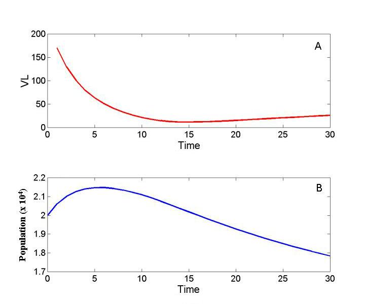
First, we show an example in which OSFA management leads to a decline of the fisheries and, eventually, of human use of the region (Figs. 10 and 11). Harvest policies are relatively permissive, the intensity parameter β is relatively high so that people move relatively quickly to more productive lakes, and travel costs are relatively low. The result is a pattern of fishery decline (Fig. 10A) followed by a decrease in the number of people using the region (Fig. 10B).
|
Fig. 10. Results of a simulation in which fishing collapses. A represents the inclusive value of the lake district (VL) vs. time, and B the human population vs. time. Parameter values are in Appendix 8.
|
|
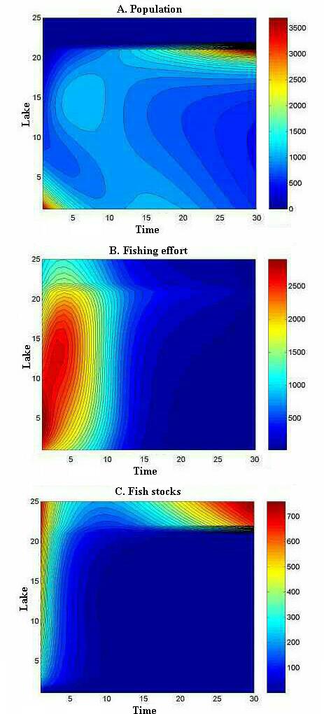
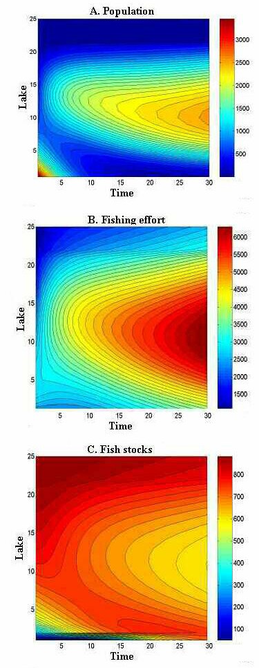
Fig. 11. Spatial dynamics in a simulation in which fishing collapses. A represents the spatial distribution of population vs. time, B of angling effort vs. time, and C of fish stocks vs. time. The lakes closest to the access point are at the lower end of the lake axis. Those farthest from the access point are wilderness lakes, unavailable for housing but available for fishing. Parameter values are in Appendix 8.
|
Contour plots show the spatial dynamics of human population, fishing effort, and fish stocks (Fig. 11). Initially, the population is concentrated near the major highway or population center (Fig. 11A). Over the first 15 yr or so of the simulation, people distribute themselves broadly among the potential base lakes. Later in the simulation, when fish stocks have declined over much of the landscape, the population is concentrated near the wilderness lakes. Fishing effort (Fig. 11B), in contrast, spreads rapidly over the landscape during the first 10 yr of the simulation, and then declines as fish populations decline. Fish stocks (Fig. 11C) decline rapidly in all lakes over the first 5 yr of the simulation. In many of the lakes with housing along the shoreline, stocks drop below the critical depensation point. After about year 20 of the simulation, fish stocks begin to recover in the wilderness lakes. This recovery is facilitated by the decline in the total number of people using the landscape.
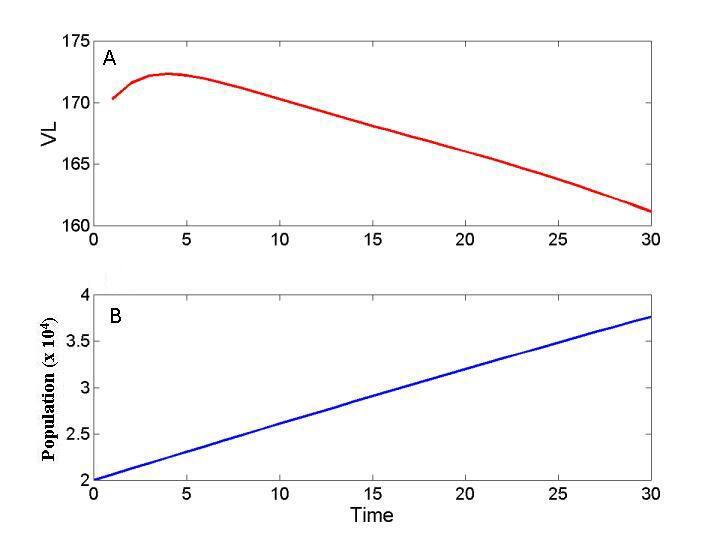
In a contrasting case, harvest regulations were less permissive; the intensity parameter β was decreased, thereby slowing the movement of people to more productive lakes; and travel costs were increased (Figs. 12 and 13). Inclusive value of the region declined somewhat over time (Fig. 12A), but this decline was not large enough to deter the continued growth of human use of the region (Fig. 12B).
|
Fig. 12. Results of a simulation in which fishing persists. A shows the inclusive value of the lake district (VL) vs. time, B of human population vs. time. Parameter values are in Appendix 8.
|
|
Fig. 13. Spatial dynamics in a simulation in which fishing persists. A shows the spatial distribution of houses vs. time, B of angling effort vs. time, and C of fish stocks vs. time. The lakes closest to the access point are at the lower end of the lake axis. Those farthest from the access point are wilderness lakes, unavailable for housing but available for fishing. Parameter values are in Appendix 8.
|
Contour plots show the spatial dynamics of people, effort, and fishes (Fig. 13). Both people and fishing effort tend to build up through the center of the spatial gradient, where anglers may access more lakes for about the same travel costs (Fig. 13). Effort grew through the simulation commensurate with the increase in human use of the area. However, harvest restrictions kept the fish stocks above the critical depensation point in most lakes. During the latter half of the simulation, fish stocks appeared to be inversely related to effort, suggesting that fishing mortality was an important factor controlling fish population density.
A rights-based management system might create a limited number of marketable access rights for the fishery (Repetto 2001, Wilson 2002). We simulated such a system by holding the human population constant at a level that sustained a relatively heavy fishing effort. The system persisted for 100 yr (Fig. 14), and, in longer runs with the same parameters, the system also appeared to persist. Although the total number of people remained constant, agents were allowed to redistribute them across the landscape, approaching a gradient with more individuals near the wilderness lakes, which had higher fish populations, and fewer people near the major highway or population center. Angling effort shifted toward the middle of the spatial gradient, as noted in previous simulations. Fish stocks collapsed and never recovered in the lake nearest to the main highway or population center. Among the other lakes, fish stocks were lowest near the center of the gradient but remained above the critical depensation point. Fish stocks were highest in the wilderness lakes.
Effects of dual management regimesSome landscapes are managed with a few different regimes that recognize important differences among broad classes of lakes. One example of such a system is the walleye (Stizostedion vitreum) co-management system used by the State of Wisconsin and the Lake Superior Chippewa Nation (Loew 2001) for the Ceded Territories of Wisconsin (Beard et al. 2003b). We simulated a dual management regime that is a caricature of this co-management system. We did not attempt to represent all the details of the actual co-management system. For our purposes, the essential feature is that co-managed lakes are subject to strict regulations that are intended to ensure that the population of adult game fish does not drop below a specified minimum number (Beard et al. 2003b). Thus, our goal is to compare a landscape with a single management regime to a landscape with dual management regimes under which some of the lakes are subject to different regulations.
To illustrate the effects of dual management regimes, we designed our simulations with liberal bag limits on most lakes and an escapement system on co-managed lakes. In our model, 20% of the lakes were subject to co-management. Under co-management, the escapement system attempted to maintain at least 300 adult fish/ha by the end of each season by limiting the sum of harvest by anglers plus tribal fishers.
Dual management substantially increased the inclusive value of the region and thereby increased the growth of the human population (Fig. 15). Spatial dynamics were more complex than in previous simulations (Fig. 16). During the first 5 yr of the simulation, fish stocks were lower in the co-managed lakes; see gradient position 11-15. As the number of people and effort rise, fish stocks decline in the lakes that are not co-managed, while stocks remain roughly constant in the co-managed lakes. As a consequence, the fish stocks in the co-managed lakes are larger than those in the neighboring lakes subject to more liberal harvest regulations. Near the end of the simulation, the fish populations of the wilderness lakes have declined to about the level found in the co-managed lakes. Fishing effort grows through the simulation as the human population grows. Near the end of the simulation, effort is larger near the co-managed lakes. In part, this is because people tend to congregate near the co-managed lakes.
These simulations are merely a caricature of the situation in Wisconsin and have some unrealistic features. For example, land management decisions by the Chippewa Nation may limit housing development around some co-managed lakes (Peterson et al. 2003a), leading to distributions of housing and effort that are considerably different from the simulation shown here. The actual spatial pattern of residents and visitors, as well as the spatial distribution of co-managed lakes, are considerably more complicated than the pattern represented by these simulations.
Despite their simplicity, these simulations do show that multiple management regimes may considerably increase the inclusive value of a region. In the simulations, this occurs because multiple management regimes enable more lakes to be managed by more nearly optimal policies. Even a simple diversification of management regimes can significantly increase the inclusive value of a recreational landscape of lakes.
Summary of the simulationsPolicy analysis for the multiple-lake case shows that policies should consider differences among individual lakes. The simulations show that neglect of interlake variation can lead to substantial losses of social welfare and serial collapses of sport fisheries. At the level of each individual lake, policies should seek to promote the persistence of the game fish populations. There is risk of domino effects if the collapse of the fish population in one lake causes anglers to move to neighboring lakes, leading to declines in those fish populations. Thus, management of the region as a whole must take account of the mobility of the anglers. Relatively cautious regulations that promote the persistence of fish populations in all lakes may sacrifice utility, thereby decreasing the attractiveness of the lake district to potential visitors. On the other hand, overly liberal regulations may lead to local stock collapses and domino effects that may severely decrease the attractiveness of the lake district as a whole. The manager is challenged at multiple scales.
The size of the angler population is a critical variable in determining fish dynamics and related policies. If the manager derives revenue from fishing activity, there is a natural tendency to promote the fishery. Such promotion invites the very overexploitation that could destroy the attractiveness of the lake district.
The simulations suggest some ways to build the economy of the lake district without crashing the fisheries. Diversification of management regimes is important. Even a simple differentiation among categories of lakes is helpful if it facilitates a match between policies and lake-specific conditions. For example, catch-and-release policies could be implemented on at least some lakes that meet certain criteria. In sport fisheries, such policies separate catch from harvest. Catch rates can be high, perhaps increasing angler satisfaction, while mortality rates remain low.
The optimal policy is highly heterogeneous in space and variable over time. A rights-based system could lead naturally to the emergence of endogenous, self-organized, lake-specific management that would improve the inclusive value for the landscape as a whole. Conditions for the development of such systems are reviewed by Ostrom et al. (2002).
A form of diversification that we have not explored in this paper is to expand the economy in dimensions other than fishing. In model terms, this implies increasing the dimensionality and magnitude of A0i. Clearly, such expansion could increase the inclusive value of the lake district. However, the opposite could occur if the expansion of A0i led to a breakdown of ecosystem services, which would correspond to fishery collapse in our model. Regions dependent on ecosystem recreation face the challenge of diversifying the economy without compromising the ecosystem services on which the economy depends.
This paper explores a system of rational, mobile agents using an ecosystem service on a heterogeneous landscape. We sought a model that was complex enough to represent essential processes, yet simple enough to understand. Like all models, the one in this paper has strengths and weaknesses.
The model uses a familiar framework for economic choices by rational agents. The ecosystem model represents a lake fishery subject to depensation and trophic cascades and responsive to harvest and habitat modification by humans. For the deterministic case of a rational point expectations equilibrium, we compute optimal fisheries management policies. Even for this simplified situation, the optimal policies are considerably more complicated than the policies commonly used by agencies that manage sport fisheries. It is possible that a rights-based system could lead to endogenous mechanisms that approximate the optimal policies. By simulation, we show how the dynamics of each lake's fishery are coupled to the fisheries of neighboring lakes through the activities of mobile anglers. These analyses expose the complexity of the task before fish managers. They must maintain the economic benefits from a regional ecosystem service in the context of exogenous economic forces while sustaining the resource on a diverse landscape of lakes with individualistic dynamics.
By focusing the model on a single lake district over time horizons of a few decades, we have omitted some important processes. Demographic, political, and economic changes in the larger environment will affect any lake district. In our model, these large external forces are condensed into a single parameter that represents the inclusive value of some alternative destination to which people may migrate. The model ignores long-term changes in the social preferences that affect fishing, although such changes could be approximated by converting some of the model's parameters to variables. For example, innovations in fishing technology could be represented by a gradual increase in catchability (q), or changes in the satisfaction derived from catching fish could be represented by gradual changes in the exponent of the utility function (a). The model also ignores long-term changes in ecological factors such as climate change, forest dynamics, and invasions of exotic species. Such long-term changes could be represented by converting ecological parameters to slowly changing variables.
Other simplified features of our social-economic model should be noted. We represented the optimal policy by a rational point expectations equilibrium. As seen in the simulations, the model exhibits decadal changes that may cause an equilibrium approach to be suboptimal. A more dynamic policy will be even more complicated than the one obtained for rational point expectations equilibrium. This reinforces our conclusion that the optimal fisheries policy for a lake district is substantially more heterogeneous and lake-specific than the policies typically adopted in sport fish management.
We have assumed that agents know the correct model for the sport fishery, know parameter values precisely, and observe the fish population with negligible errors. These assumptions are highly unrealistic. Much of the scientific literature of fisheries is devoted to analyzing uncertainty and its consequences for policy choice (Ludwig 1995, Walters 1986, Hilborn and Walters 1992). In models of management for a single lake, the dynamics of uncertainty play a central role in complex changes of social-ecological systems (Carpenter et al. 1999, Carpenter 2002, Peterson et al. 2003b). Future research on uncertainty and learning using our model will probably expose new complexities.
From the enormous diversity of potential ecosystem models, we have chosen a model that represents minimal features of fish population dynamics, including critical depensation, dependency of recruitment on habitat, effects of harvest, and the possibility of stock persistence under some harvest regimes. Our model also exhibits trophic cascades, which link fish dynamics to water quality (Carpenter 2003). On the other hand, our model does not include the multiplicity of life-history characteristics found in keystone predators of actual lakes and does not address the possibility of fishing on multiple species. These complexities were excluded in an effort to produce a tractable and understandable model.
Habitat emerges as an important variable for fisheries management on the landscape. The dynamics of habitat are slower than those of the fishery (Turner 2003). Our model for habitat effects is simple and stylized. The most unrealistic feature is the symmetric response of habitat to changes in the population of shoreline residents. In real lakes, removal of habitat such as fallen trees can occur within a few years, whereas replacement of this habitat may take hundreds of years (Christensen et al. 1996, Turner 2003). Future research on this topic should include the slow dynamics of habitat in the model, as well as economic factors related to habitat management.
Insights from the modelSpatial dynamic models of marine fisheries show waves of underharvest and overharvest that resemble the domino effects demonstrated here (Sanchirico and Wilen 1999, 2001). Similar models address the value of marine reserves, which are in some ways analogous to the dual management regimes considered in this paper (Sanchirico and Wilen 1998, Walters 2000). Our work adds three new features to this existing literature:
- Lake fish stocks are spatially isolated, so that the movements of fishes that contribute to spatial equilibration in marine systems are absent in lakes.
- The insularity of lake fish stocks exacerbates their vulnerability to collapse, represented by depensation in our model. The vulnerability of lake fish stocks seems to be related to food web processes and habitat destruction (Post et al. 2002, Schindler and Scheuerell 2002). Both phenomena are represented in our model.
- In sport fisheries, there is a slow component of angler movement related to choice of lake districts and choice of base lake within a lake district, as well as a fast component related to movement among lakes near the base lake. Marine fishing fleets, in contrast, are usually thought to rapidly adjust to spatial patterns of fishing opportunity (Gillis et al. 1993). Our model represents both the slow and fast components of fisher dynamics. As a consequence of these three differences, the spatial dynamics shown in this paper are different from those seen in marine models. In particular, lake fisheries can collapse, and localized collapse combined with slow movements of fishers can lead to persistent spatial patterns in the fisheries of a landscape. Although the management of such patterns poses some of the same difficulties as the marine case, the managers of lake fisheries can consider tools such as habitat regulations and hatchery stocking, in addition to harvest regulation.
The microeconomic analysis of sport-angler behavior suggests that effort should be proportional to fish population size raised to a positive exponent possibly near 1. This finding provides an economic rationale for the models of sport fishing mortality used by previous authors (Beard et al. 2003b, Cox et al. 2003).
Ecologists have often noted that even relatively simple food-web structures can create the possibility of multiple dynamic regimes, including depensatory crashes (Walters and Kitchell 2001, de Roos and Persson 2002, Carpenter 2003). The trophic triangle model presented in this paper is a simple, tractable way of representing such dynamics, yet retains key biotic parameters related to recruitment, size-dependent predation, and effects of habitat on trophic interactions. The model also represents trophic cascades. Because this model combines simplicity, parameters grounded in biology, and certain types of interesting dynamics, it may be useful for a wider range of applications.
Habitat is a second dimension for policy that may have advantages over harvest regulation in some situations. Habitat improvement increases the resilience of game fish populations, meaning that the populations can experience larger shocks without crossing the critical depensation point. Habitat improvements also make it possible to relax harvest regulations. Choices by individual unregulated agents become more similar to the choices preferred by society as a whole. In this sense, social resilience increases as well. The slow dynamics of habitat give agencies a policy lever that may have long-lasting benefits (Turner 2003).
Spatial patterns of angler access and lake-specific ecology have powerful implications for sport fish management. For example, movements of anglers can create local stock collapses that spread like falling dominoes across a landscape. Such collapses are made more likely by one-size-fits-all (OSFA) policies, which are common in regional sport fish management. On the other hand, there are significant costs in designing and implementing lake-specific policies. Moreover, the lake-specific policies should change over time as social and ecological conditions change.
Collectively, these patterns cast doubt on the idea that lake sport fisheries are independent systems largely stabilized by endogenous regulation. Most sport fisheries are managed using OSFA regulations intended to provide some minimal level of protection for fish stocks (Noble and Jones 1993, Radomski et al. 2001, Beard 2002). These management regimes often fail to achieve predicted outcomes for reasons that include insufficiently stringent regulations (Cook et al. 2001, Radomski et al. 2001) and illegal harvest (Gigliotti and Taylor 1990). In regions with many lakes and mobile anglers, one would expect all fish stocks to approach a level that provided constant opportunity for anglers across the landscape (Cox and Walters 2002, Cox et al. 2003). Our microeconomic model of angler behavior supports this expectation. In addition, our model shows how travel costs, nonangling opportunities, housing markets, and competing opportunities in other regions can lead to more complex spatial phenomena.
All of this work, however, supports the conclusion that fisheries on a set of lakes are co-dependent. From a manager's point of view, the possibility of dominolike decreases in fish stocks, leading to regionally degraded fisheries like those studied by Post et al. (2002), is especially alarming. OSFA regulations are susceptible to such dynamics. If regulation is insufficiently stringent, fish declines on less resilient lakes can lead to increased effort followed by stock declines on nearby lakes. If regulation is too stringent, incentives for illegal harvest may also lead to landscape-wide degradation of fisheries. Thus, by eroding either ecological or social resilience, OSFA creates landscape-scale vulnerability.
A rights-based system (Repetto 2001, Wilson 2002) may perform better than OSFA regulations by allowing the endogenous organization of lake-specific practices. In sport fisheries, however, public access is a long-standing tradition. Devolution of property rights from the state to lake-specific ownership of catch quotas represents a significant departure from this tradition. Groups who see themselves as likely losers will oppose such devolution. To ensure that certain groups are not excluded from the fishery, novel mechanisms for allocating rights, such as lotteries for lake-specific quotas, may be necessary.
A rational social planner for a lake district faces challenges on multiple scales. On one level, the inclusive value of the region depends on its ability to attract more people than other regions that offer different bundles of benefits. At the same time, the growth in the human population places pressures on ecosystem services that could diminish them and thereby reduce the inclusive value of the region. Movement of agents within the region can create local instabilities of ecosystem services and cause the instabilities to spread across the landscape. Heterogeneity of ecosystems suggests that policy must also be heterogeneous. Moreover, policies must be flexible enough to adapt to long-term changes in social and ecological variables. These considerations suggest that diversity of policy options and economic opportunity should be combined with devolution of property rights to the local level to increase the long-term inclusive value of lake districts.
How much disaggregation of management is appropriate? Although we have demonstrated important costs and inefficiencies in OSFA, one must remember that lake-specific management will also have costs. For example, lake-specific policies will require much more effort in assessing and sanctioning to enforce regulations. Individual fishers' costs would go up because of the need to know the regulations on each different lake. There may be economies of scale that are lost by replicating management institutions for each lake. For example, fish stock assessment is an expensive technological exercise that may be handled more efficiently by regional institutions. Thus, between the extremes of OSFA and completely disaggregated management, there should be some intermediate level of aggregation that produces the best results (Low et al. 2002). Our model provides a framework for exploring the consequences for regional inclusive value and ecosystem services that result from different degrees of aggregation or disaggregation of policies.
The formation of a lake-specific management unit is related to the work of Brock and de Zeeuw (2002), who explore the conditions for cooperation in a repeated game in which many users exploit an ecosystem service subject to catastrophic collapse. Under certain conditions it makes sense for resource users to organize to limit resource use by individuals to avoid long-term losses. These could be viewed as minimal conditions for formation of a management association at the scale of a single lake within the landscape. Additional social factors necessary for the creation of an effective co-management institution are addressed by Ostrom (1990) and Ostrom et al. (2002). Related ideas applied to the specific case of lake water quality management are discussed by Scheffer et al. (2000).
Our analysis begs the question of learning about spatially heterogeneous social-ecological systems subject to complex dynamics. The challenge of learning about such systems is at the heart of natural resource policy. Landscapes have stochastic dynamics, social-ecological data have large uncertainties, and all natural resource management models are mis-specified. These complications cause learning to be slow. Slow learning introduces social and economic instabilities (Brock and Hommes 1997). In the case of ecosystems, slow learning makes overexploitation and collapse more likely (Walters 1986, Carpenter 2003, Peterson 2003b). Therefore, learning by heterogeneous agents co-managing landscapes of stochastic nonlinear ecosystems is an important frontier for future research. We believe that the approach introduced in this paper offers a promising framework.
We plan further work of two kinds. First, it is natural to extend the current model to include stochasticities and uncertainties. This process has been initiated for trophic triangle models (Carpenter 2003), but far more work is needed to integrate the ecological dynamics with more realistic models of agent behavior. Second, we are developing a version of the model that can be played as a game to study learning and the dynamics of decision making by real people attempting to co-manage simulated landscapes. We hope that a combination of theoretical and practical research based on the general approach described in this paper will contribute to a broader understanding of spatially heterogeneous social-ecological systems.
Responses to this article are invited. If accepted for publication, your response will be hyperlinked to the article. To submit a comment, follow this link. To read comments already accepted, follow this link.
We thank T. D. Beard and G. D. Peterson for discussions of theory and practice for spatially heterogeneous fisheries. T. D. Beard, S. P. Cox, and two anonymous referees wrote helpful reviews of the draft manuscript. Our work is supported by the National Science Foundation and the J. S. MacDonnell Foundation through a grant to the Resilience Alliance. In addition, W. A. Brock's work is supported by the Vilas Trust.
Allen, P. M., and J. M. McGlade. 1987. Modeling and complex human systems: a fishery example. European Journal of Operations Research 30:147-167.
Anderson, S., A. de Palma, and J. Thisse. 1992. Discrete choice theory of product differentiation. MIT Press, Cambridge, Massachusetts, USA.
Axelrod, R. 1997. The complexity of cooperation. Princeton University Press, Princeton, New Jersey, USA.
Beard, T. D. 2002. The roles of recruitment, angler effort response, angler perception, and exploitation limits in structuring regional walleye fisheries in northern Wisconsin. Dissertation. University of Wisconsin-Madison, Madison, Wisconsin, USA.
Beard, T. D., Jr., S. P. Cox, and S. R. Carpenter. 2003a. Impacts of daily bag limit reductions on angler effort in Wisconsin walleye lakes. North American Journal of Fisheries Management 23, in press.
Beard, T. D., Jr., P. W. Rasmussen, S. P. Cox, and S. R. Carpenter. 2003b. Evaluation of a mixed walleye spearing and angling fishery management system in northern Wisconsin. North American Journal of Fisheries Management 23, in press.
Becker, G. 1991. A treatise on the family. Harvard University Press, Cambridge, Massachusetts, USA.
Beisner, B. E., C. L. Dent, and S. R. Carpenter. 2003. Variability of lakes on the landscape: roles of phosphorus, food webs and dissolved organic carbon. Ecology 84:1563-1575 .
Biro, P. A., J. R. Post, and E. A. Parkinson. 2003. From individuals to populations: prey fish risk-taking mediates mortality in whole-system experiments. Ecology 84:2419-2431.
Bockstael, N. E. 1996. Modeling economics and ecology: the importance of a spatial perspective. Journal of Agricultural Economics 78:1168-1180.
Brander, J., and M. Taylor. 1997. International trade between consumer and conservationist countries. Resource and Energy Economics 18:267-298.
Brock, W. 1972. On models of expectations that arise from maximizing behavior of economic agents over time. Journal of Economic Theory 5(3):348-376.
Brock, W. A., and A. de Zeeuw. 2002. The repeated lake game. Economics Letters 76:109-114.
Brock, W. A., and C. H. Hommes. 1997. A rational route to randomness. Econometrica 65:1059-1095.
Brock, W. A., and J. A. Scheinkman. 1985. Price-setting supergames with capacity constraints. Review of Economic Studies 52:371-382.
Brooks, J. L., and S. I. Dodson. 1965. Predation, body size, and composition of plankton. Science 150:28-35.
Brown, G. M., and J. Roughgarden. 1997. A metapopulation model with private property and a common pool. Ecological Economics 22:65-71.
Carpenter, S. R. 2002. Ecological futures: building an ecology of the long now. Ecology 83:2069-2083.
Carpenter, S. R. 2003. Regime shifts in lake ecosystems: pattern and variation. Excellence in Ecology Series, Volume 15. Ecology Institute, Oldendorf/Luhe, Germany.
Carpenter, S. R., W. A. Brock, and P. C. Hanson. 1999. Ecological and social dynamics in simple models of ecosystem management. Conservation Ecology 3(2):4. [online] URL: http://www.consecol.org/vol3/iss2/art4.
Carpenter, S. R., A. Muñoz del Río, S. Newman, P. Rasmussen, and B. M. Johnson. 1994. Interactions of anglers and walleyes in Escanaba Lake, Wisconsin. Ecological Applications 4:822-832.
Chichilnisky, G. 1994. North-south trade and the global environment. American Economic Review 84:427-434.
Chichilnisky, G., and G. Heal. 1993. Global environmental risks. Journal of Economic Perspectives 7:65-86.
Christensen, D. L., B. R. Herwig, D. E. Schindler, and S. R. Carpenter. 1996. Impacts of lakeshore residential development on coarse woody debris in north temperate lakes. Ecological Applications 6:1143-1149.
Cohen, J. E., T. Jonsson, and S. R. Carpenter. 2003. Ecological community description using food webs, species abundance and body size. Proceedings of the National Academy of Sciences 100:1781-1786.
Cook, M. F., T. J. Goeman, P. J. Radomski, J. A. Younk, and P. C. Jacobson. 2001. Creel limits in Minnesota: a proposal for change. Fisheries 25:19-26.
Cox, S., T. D. Beard, and C. J. Walters. 2003. Harvest control in open access sport fisheries: hot rod or asleep at the wheel? Bulletin of Marine Science 70: 749-761.
Cox, S., and C. Walters. 2002a. Modeling exploitation in recreational fisheries and implications for effort management on British Columbia rainbow trout lakes. North American Journal of Fisheries Management 22:21-34.
Cox, S., and C. Walters. 2002b. Maintaining quality in recreational fisheries: how success breeds failure in the management of open-access sport fisheries. Pages 107-119 in T. J. Pitcher and C. Hollingworth, editors. Recreational fisheries: ecological, economic and social evaluation. Blackwell Science, Oxford, UK.
Deaton, A., and J. Muellbauer. 1980. Economics and consumer behavior. Cambridge University Press, Cambridge, UK.
de Roos, A., and L. Persson. 2002. Size-dependent life-history traits promote catastrophic collapses of top predators. Proceedings of the National Academy of Sciences 99:12907-12912.
Evans, G., and S. Honkapohja. 2001. Learning and expectations in macroeconomics. Princeton University Press, Princeton, New Jersey, USA.
Flannery, T. 2002. The endless frontier. Grove/Atlantic, New York, New York, USA.
Gigliotti, L. M., and W. W. Taylor. 1990. The effect of illegal harvest on recreational fisheries. North American Journal of Fisheries Management 10:106-110.
Gillis, D. M., R. M. Peterman, and A. V. Tyler. 1993. Movement dynamics in a fishery: application of the ideal free distribution to spatial allocation of effort. Canadian Journal of Fisheries and Aquatic Sciences 50:323-333.
Gunderson, L. H., and C. S. Holling, editors. 2002. Panarchy: understanding transformation in human and natural systems. Island Press, Washington D.C., USA.
Hartley, P. 1997. Conservation strategies for New Zealand. Daphne Brasell, Wellington, New Zealand.
Heal, G. 2001. Bundling public and private goods. Available online at: http://www-1.gsb.columbia.edu/faculty/gheal/EconomicTheoryPapers/pubgoodspropvalues.pdf.
Hilborn, R., and C. J. Walters. 1987. A general model for simulation of stock and fleet dynamics in spatially heterogeneous fisheries. Canadian Journal of Fisheries and Aquatic Sciences 44:1366-1369.
Hilborn, R., and C. Walters. 1992. Quantitative fisheries stock assessment: choice, dynamics and uncertainty. Chapman and Hall, London, UK.
Hodgson, J. R., and J. F. Kitchell. 1987. Opportunistic foraging by largemouth bass (Micropterus salmoides). American Midland Naturalist 118:323-336.
Hudgins, M. D., and W. D. Davies. 1984. Probability angling: a recreational fishery management strategy. North American Journal of Fisheries Management 4:341-349.
Hunt, K. M., and R. B. Ditton. 1997. The social context of site selection for freshwater fishing. North American Journal of Fisheries Management 17:331-338.
Janssen, M. A., and S. R. Carpenter. 1999. Managing the resilience of lakes: a multi-agent modeling approach. Conservation Ecology 3(2):15. [online] URL: http://www.consecol.org/vol3/iss2/art15.
Johnson, B. M., and S. R. Carpenter. 1994. Functional and numerical responses: a framework for fish-angler interactions? Ecological Applications 4:808-821.
Keast, A. 1985. The piscivore feeding guild of fishes in small freshwater ecosystems. Environmental Biology of Fishes 12:119-129.
Levin, S. A. 1999. Fragile dominion: complexity and the commons. Perseus Books, Reading, Massachusetts, USA.
Likens, G. E. 1992. The ecosystem concept: its use and abuse. Excellence in Ecology Series, Volume 3. Ecology Institute, Oldendorf/Luhe, Germany.
Loew, P. 2001. Indian nations of Wisconsin. Wisconsin State Historical Society Press, Madison, Wisconsin, USA.
Low, B., E. Ostrom, C. Simon, and J. Wilson. 2002. Redundancy and diversity: do they influence optimal management? Pages 83-114 in F. Berkes, J. Colding, and C. Folke, editors. Navigating social-ecological systems. Cambridge University Press, Cambridge, UK.
Ludwig, D. 1995. A theory of sustainable harvesting. Journal of Applied Mathematics 55:564-575.
Ludwig, D., S. Carpenter, and W. Brock. 2003. Optimal phosphorus loading for a potentially eutrophic lake. Ecological Applications 13, in press.
Mas-Collel, A., M. Whinstin, and J. Green. 1995. Microeconomic theory. Oxford University Press, Oxford, UK.
Mather, M. E., D. L. Parrish, R. A. Stein, and R. M. Muth. 1995. Management issues and their relative priority within state fisheries agencies. Fisheries 20:14-21.
Mosindy, T. E., W. T. Momot, and P. J. Colby. 1987. Impact of angling on production and yield of mature walleyes and northern pike in a small boreal lake in Ontario. North American Journal of Fisheries Management 7:493-501.
Noble, R. L., and T. W. Jones. 1993. Managing fisheries with regulations. Pages 383-404 in C. C. Kohler and W. A. Hubert, editors. Inland fisheries management in North America. American Fisheries Society, Bethesda, Maryland, USA.
Olson, M. H., G. G. Mittelbach, and C. W. Osenberg. 1995. Competition between predator and prey: resource-based mechanisms and implications for size-structured dynamics. Ecology 76:1758-1771.
Olson, M. H., S. R. Carpenter, P. Cunningham, S. Gafny, B. R. Herwig, N. P. Nibbelink, T. Pellett, C. Storlie, A. S. Trebitz, and K. A. Wilson. 1998. Managing macrophytes to improve fish growth: a multi-lake experiment. Fisheries 23:6-12
Ostrom, E. 1990. Governing the commons: the evolution of institutions for collective action. Cambridge University Press, Cambridge, UK.
Ostrom, E., T. Dietz, N. Dolsak, P. Stern, S. Stonich, and E. Weber, editors. 2002. The drama of the commons. National Academy Press, Washington, D.C., USA.
Paine, R. T. 1980. Food webs, linkage interaction strength, and community structure. Journal of Animal Ecology 49:667-685.
Peterson, G. D., T. D. Beard Jr., B. E. Beisner, E. M. Bennett, S. R. Carpenter, G. S. Cumming, C. L. Dent, and T. D. Havlicek. 2003. Assessing future ecosystem services: a case study of the Northern Highlands Lake District, Wisconsin. Conservation Ecology 7(3):1. [online] URL: http://www.consecol.org/vol7/iss3/art1.
Peterson, G. D., S. R. Carpenter, and W. A. Brock. 2003. Uncertainty and management of multi-state ecosystems: an apparently rational route to collapse. Ecology 84, in press.
Post, J. R., M. Sullivan, S. P. Cox, N. P. Lester, C. J. Walters, E. A. Parkinson, A. J. Paul, L. Jackson, and B. J. Shuter. 2002. Canada's recreational fisheries: the invisible collapse? Fisheries 27:6-17.
Radomski, P. J., G. C. Grant, P. C. Jacobson, and M. F. Cook. 2001. Visions for recreational fishing regulations. Fisheries 26:7-18.
Redman, C. L. 1999. Human impact on ancient environments. University of Arizona Press, Tucson, Arizona, USA.
Repetto, R. 2001. A natural experiment in fisheries management. Marine Policy 25:251-264.
Sanchirico, J. N., and J. E. Wilen. 1998. Marine reserves: is there a free lunch? Resources for the Future Working Paper Number 99-09. Resources for the Future, Washington, D.C., USA.
Sanchirico, J. N., and J. E. Wilen. 1999. Bioeconomics of spatial exploitation in a patchy environment. Journal of Environmental Economics and Management 37:129-150.
Sanchirico, J. N., and J. E. Wilen. 2001. Dynamics of spatial exploitation: a metapopulation approach. Natural Resources Modeling 14:391-418.
Sargent, T. 1993. Bounded rationality in macroeconomics. Oxford University Press, Oxford, UK.
Scheffer, M., W. Brock, and F. Westley. 2000. Socioeconomic mechanisms preventing optimum use of ecosystem services: an interdisciplinary theoretical analysis. Ecosystems 3:451-471.
Schindler, D. E., S. I. Geib, and M. R. Williams. 2000. Patterns of fish growth along a residential development gradient in north temperate lakes. Ecosystems 3:229-237.
Schindler, D. E. and M. D. Scheuerell. 2002. Habitat coupling in lake ecosystems. Oikos 98:177-189
Schindler, D. E., J. R. Hodgson, and J. F. Kitchell. 1997. Density-dependent changes in individual foraging specialization of largemouth bass. Oecologia 110:592-600.
Tonn, W. E., and J. J. Magnuson. 1982. Patterns in the species composition and richness of fish assemblages in northern Wisconsin lakes. Ecology 63:1149-1166.
Turner, M. G. 2003. Modeling for synthesis and integration: forests, people and riparian coarse woody debris. Pages 83-111 in C. Canham and W. Lauenroth, editors. Understanding ecosystems: the role of quantitative models in observation, synthesis and prediction. Princeton University Press, Princeton, New Jersey, USA.
Turner, M. G., R. H. Gardner, and R. V. O'Neill. 2001. Landscape ecology in theory and practice. Springer-Verlag, New York, New York, USA.
Ursin, E. 1982. Stability and variability in the marine ecosystem. Dana 2:51-65.
Varian, H. 1992. Microeconomic analysis. Third edition. Norton, New York, New York, USA.
Walters, C. J. 1986. Adaptive management of renewable resources. MacMillan, New York, New York, USA.
Walters, C. J. 2000. Impacts of dispersal, ecological interactions and fishing effort dynamics on efficacy of marine protected areas: how large should protected areas be? Bulletin of Marine Science 66:745-759.
Walters, C., and J. F. Kitchell. 2001. Cultivation/depensation effects on juvenile survival and recruitment: implications for the theory of fishing. Canadian Journal of Fisheries and Aquatic Sciences 58:1-12.
Werner, E., and J. F. Gilliam. 1984. The ontogenetic niche and species interactions in size-structured populations. Annual Review of Ecology and Systematics 15:393-425.
Werner, E. E., J. F. Gilliam, D. J. Hall, and G. G. Mittelbach. 1983. An experimental test of effects of predation risk on habitat use in fish. Ecology 64:1540-1548.
Wilson, J. A. 2002. Scientific uncertainty, complex systems and the design of common-pool institutions. Pages 327-359 in E. Ostrom, T. Dietz, N. Dolsak, P. Stern, S. Stonich, and E. Weber, editors. The drama of the commons. National Academy Press, Washington, D.C., USA.
| Symbol | Subscript |
Unit |
Explanation |
||||||||||||||||||||||||||
| β | ... |
Dimensionless | Intensity of choice parameter for choosing a base lake | ||||||||||||||||||||||||||
| ε | ... |
Dimensionless | Parameter for adjusting the flux rate of people into or out of the lake district | ||||||||||||||||||||||||||
 |
... |
People/inclusive value | Parameter for strength of preference for choosing the lake district versus alternate destinations | ||||||||||||||||||||||||||
| λ | ... |
... |
LaGrange multiplier | ||||||||||||||||||||||||||
| Λ | ... |
... |
LaGrangian function | ||||||||||||||||||||||||||
| τ | Base lake, lake fished | Lake | Time allocation to an activity by a person | ||||||||||||||||||||||||||
| a | ... |
Dimensionless | Exponent for Cobb-Douglas production function; 0 < a < 1. | ||||||||||||||||||||||||||
| A | Lake, time | Fish/lake | Adult game fish population | ||||||||||||||||||||||||||
| A0 | Lake | Fish/lake | Potential benefit from alternative, non-fishing activity | ||||||||||||||||||||||||||
| b | ... |
Dimensionless | Exponent used in calculating time allocation; b = a /(1-a) | ||||||||||||||||||||||||||
| c | Prey type | Predator/time | Predation coefficient on forage fish or juvenile game fish | ||||||||||||||||||||||||||
| C | Base lake, lake fished | Lake/cost | Inverse travel cost for fishing a particular lake by a representative person based on a given lake | ||||||||||||||||||||||||||
| D | Lake | Utility | Cost of being based on a particular lake | ||||||||||||||||||||||||||
| E | Lake, time | Time | Effort, i.e. total time spent fishing by a population of anglers | ||||||||||||||||||||||||||
| f | ... |
Juveniles/adult | Annual fecundity of adult game fishes | ||||||||||||||||||||||||||
| F | Time | Fish/lake | Forage fish population | ||||||||||||||||||||||||||
| g | ... |
Time | Growth rate of the forage fish population | ||||||||||||||||||||||||||
| h | ... |
Time | Hiding or refuging rate coefficient for juvenile game fish | ||||||||||||||||||||||||||
| J | Vulnerable or hiding; time | Fish/lake | Juvenile game fish population | ||||||||||||||||||||||||||
| m | ... |
adult/time | Density-dependent mortality coefficient for game fish; maximum game fish population » 1/m | ||||||||||||||||||||||||||
| M | Fish, lake, time | Fish/time | Mortality rate of fish | ||||||||||||||||||||||||||
| N | Lake, time (or the entire lake district) | People | Number of people | ||||||||||||||||||||||||||
| p | Base lake, lake fished | Utility/fishing time | Tax-equivalent policy parameter for regulation of fishing | ||||||||||||||||||||||||||
| q | ... |
Time/effort | Catchability | ||||||||||||||||||||||||||
| r | ... |
... |
Exponent in Constant Elasticity of Substitution model; elasticity = 1/(1-r). | ||||||||||||||||||||||||||
| R | Ecological or social | Dimensionless | Resilience | ||||||||||||||||||||||||||
| s | ... |
Dimensionless | Overwinter survivorship of adult game fish | ||||||||||||||||||||||||||
| S | ... |
Utility/fishing time | Shadow price of fishing | ||||||||||||||||||||||||||
| t | ... |
Time | Time | ||||||||||||||||||||||||||
| T | ... |
Time | Total time available to a representative person | ||||||||||||||||||||||||||
| u | ... |
Log (forage fish)/ log (game fish) | Constant representing the slope of a log-log plot of forage fish population versus game fish population | ||||||||||||||||||||||||||
| U | Lake or time | Utility | Utility to a representative person from a specified set of activities | ||||||||||||||||||||||||||
| v | ... |
Time | Vulnerability rate coefficient for juvenile game fishes | ||||||||||||||||||||||||||
| v | Lake | Net utility | Net value of a vacation on a particular lake | ||||||||||||||||||||||||||
| V | L,O | Inclusive value | Inclusive value of a vacation in the lake district (L) or an alternate destination (O) | ||||||||||||||||||||||||||
| w | ... |
Log (forage fish) | Constant representing the intercept of a log-log plot of forage fish population vs. game fish population | ||||||||||||||||||||||||||
| W | ... |
Utility | Welfare of a representative angler, to be maximized by fishing policy | ||||||||||||||||||||||||||
| y | ... |
Time | Elapsed time during a fishing season | ||||||||||||||||||||||||||
| Z | Lake | Utility | Production of utility from a particular activity, such as fishing on a particular lake | ||||||||||||||||||||||||||
FOR INDIVIDUAL AGENTS
We use a Constant Elasticity of Substitution (CES) model for the various recreational activities of the lake users. Under this model, the total utility of a representative lake user based on lake j is
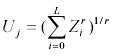 |
(A2.1) |
We will assume that the Zi are produced by Cobb-Douglas functional forms, which are often used in economics. They display many desirable properties such as (1) diminishing returns for modeling an important class of production phenomena; (2) constant factor shares under competitive pricing for modeling the production side, i.e., the supply side, of the economy; and (3) constant expenditure shares for modeling the demand side of the economy. The latter two properties are useful when confronting production models with the aggregated data common in economics. Deaton and Muellbauer (1980) provide an extensive discussion and application of CES functional forms and Cobb-Douglas functional forms to economics, especially on the demand side of the economy. Varian (1992) offers more on Cobb-Douglas and CES functional forms, especially typical uses of Cobb-Douglas functional forms in empirical work in economics.
The property of Cobb-Douglas functional forms that interests us is the diminishing returns property, i. It is natural in the household production approach to utility theory that we are using here to assume that production of each good, i.e., Zio[qAiCijτij]a that enters utility Uj in Eq. A1.1 would display diminishing returns to the production input [qAiCijτij]. One way to capture the diminishing returns property for output y = f(x) where x is input is to assume y = Axa for some positive constant a, 0 < a < 1. The function y = Axa, 0 < a < 1 is a Cobb-Douglas form that displays diminishing returns, and that is the form we are using in Eq. A2.2 below.
Thus we assume that the Zi follow Cobb-Douglas production functions. Then we can write
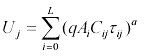 |
(A2.2) |
Time available for fishing and other activities is finite and given by
 |
(A2.3) |
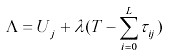 |
(A2.4) |
 |
(A2.5) |
 |
(A2.6) |
 |
(A2.7) |
 |
(A2.8) |
where the exponent b is b = a/(1-a). In Eq. A2.8 for time spent at base lake j, the summation goes from 1 to L but skips j. To account for nonfishing activities at the base lake, an additional term (AoCij)b is included in Eq. A2.1. Ao represents the reward from the nonfishing activity in fish equivalents.
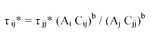 |
(A2.9) |
THE TROPHIC TRIANGLE
We will write differential equations for the dynamics of juvenile piscivores, forage fishes, and adult piscivores during the season, and integrate them over the season to obtain expressions for conditions at the beginning of the next season. Season is indexed by subscript t and elapsed time within the season is indexed by subscript y (range 0 to 1). The differential equations are
|
dAt,y/dy = -qE(At,o) At,y
|
(A3.1) |
|
dFt,y / dy = g Ft,y - cF At,y Ft,y
|
(A3.2) |
|
dJt,y / dy = - m Jt,y At,y - cJ v Ft,y Jt,y /(h + v + cJ Ft,y)
|
(A3.3) |
Equations A3.1 to A3.3 assume that, within the season, the population dynamics of A is controlled by fishing mortality rather than food supply, and that the population dynamics of F and J are controlled by predation, not food supply. Between bouts of reproduction, populations of A and J can only decrease, and we assume that harvest and predation determine the rate of decline. We assume that the metabolic needs of the surviving fishes are met by many prey items, including prey not explicitly represented in the model. Frequently, fishes are omnivores, eating preferred prey when it is available and less preferred prey otherwise (Keast 1985, Hodgson and Kitchell 1987, Schindler et al. 1997). We assume that A eat F when F are available, and otherwise they eat something else. We make the analogous assumption for F with respect to consumption of J.
During the season, fishing causes the population of adult piscivores A to decline (Eq. A3.1). In the usual theory of fishing, the mortality of adult game fish is the product of catchability q, effort E, and fish population A (Hilborn and Walters 1992). In our system, the dynamics of angler behavior cause effort to be a function of A (Appendices 2 and 5).
Forage fish dynamics are assumed to follow a simple Lotka-Volterra model with a linear functional response (Eq. A3.2).
Fig. A3.1. Schematic diagram of vulnerability, refuge-seeking behavior, and predation upon juvenile game fish.
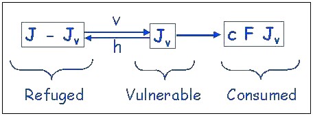
Juvenile piscivore dynamics depend on the availability of refugia and the vulnerability of juveniles to predation (Fig. A3.1). We assume that J make behavioral choices that balance foraging opportunity vs. risk of death by predation (Werner et al. 1983, Werner and Gilliam 1984, Olson et al. 1995, Biro et al. 2003). These behavioral choices are rapid, occurring many times each day. Over a short period of time during the growing season, changes in the population of juvenile game fishes vulnerable to predation by forage fishes follow Cox and Walters (2002):
|
dJv / dt = v (J - Jv) - h Jv - cJ Ft Jv
|
(A3.4) |
Because behavioral fluxes (vulnerability and hiding) are rapid compared to predation, it is reasonable to solve for the equilibrium value of Jv* = vJ/(h + v + cJFt). Thus, the predation flux of juvenile game fish to forage fish is cJFJv* = cJvFtJ/(h + v + cJFt). This expression appears as the predation loss term in Eq. A3.3.
In the multilake model simulations (Figs. 7–16), we calculate h as a sigmoid function of the number of people resident around the lake. Lakeshore residents tend to degrade fish habitat (Christensen et al. 1996, Schindler et al. 2000). Thus, h takes on relatively high values when the number of residents is low, and low values when the number of residents is high. Details are provided in Appendix 8.
The initial conditions at the beginning of a season (y = 0) are
|
At,0 = s At-1,1
|
(A3.5) |
|
Ft,0 = constant
|
(A3.6) |
|
Jt,0 = f s At-1,1
|
(A3.7) |
In the above expressions, s is overwinter survival, and f is fecundity per adult. We assume that F is able to persist at a level that yields a constant Ft,0 at the beginning of each season. For example, there could be a source population in a connected stream or lake that recolonizes the subject lake each year (Tonn and Magnuson 1982). Alternatively, there could be a small refuge within the lake that enables a small number of forage fishes to persist over each winter.
All of these assumptions could be relaxed, leading to a more complicated food-web model that could be studied, probably by simulation. Our goal, however, is to study the spatial dynamics of fishes and people using a model that is as simple as possible but still exhibits the relevant qualitative dynamics. The relevant dynamics include the possibility of depensatory collapse, the possibility of a persistent piscivore stock, and appropriate sensitivity of the piscivore dynamics to fishing and habitat. These features are present in the simplified model that we studied.
Next we derive the difference equation for projecting the adult piscivore population from one season to the next.
At any time within the season, the number of adults is obtained by integrating Eq. A3.1 to obtain
|
At,y = At,0 exp[-q E(At,0) y] = s At-1,1 exp[-q E(At,0) y]
|
(A3.8) |
Equipped with Eq. A3.8, integrate Eq. A3.2 within the season to obtain
|
Ft,y = Ft,0 exp[g y - (cF / q E(At,0)) (At,0 - At,y) ]
|
(A3.9) |
Now, Eqs. A3.8 and A3.9 are inserted into Eq. A3.3, which is solved numerically over the season to calculate Jt,1, the number of juveniles that survive to the end of the season. Thus, the number of piscivores present at the end of the season is
|
At,1 = Jt,1 + s At-1,1 exp[-q E(At,0)]
|
(A3.10) |
The number of piscivores present at the start of the next season is the number that survive the winter, or
|
At+1,0 = s At,1 = s{ Jt,1 + s At-1,1 exp[-q E(At,0)]}
|
(A3.11) |
Equation A3.11 was used to calculate the fish dynamics reported in the text.
Suppose we wish to implement τ**, the manager's choice of optimal time allocation for each angler. As a purely analytical matter, we may implement τ** by the device of a tax of p per unit effort spent angling. To discuss this as a matter of pure theory, we must define the notion of equilibrium with which we are working. We describe a rational point expectations equilibrium. Suppose each angler forms a deterministic point expectation on the number of fish in the lake at the beginning of the season and chooses effort based upon this point expectation by solving the following problem. Maximize {(qAt,0τ)a - Sτ} over τ. Here At,0 is the angler's deterministic point expectation.
In this solution, each angler fishes at a constant rate over the season. This leads to a total effort at the constant level
|
E(At,0)
 At,0) At,0)
|
(A4.1) |
for each time y of season t where y ranges from 0 to 1. Note that we assume that the expected number of fish, At,0, at the beginning of the season, t, that determines each angler's effort turns out to be the actual number of fish at the beginning of season t, i.e., we have assumed "rational" or "consistent" expectations. This device, although unrealistic in the case of sport fisheries, is a natural baseline from which to erect a theory of learning that we save for future research. See Brock (1972) for an early discussion of a theory of learning rational expectations in a different context. A recent treatment with learning theories is in Sargent (1993). This completes the description of the equilibrium notion of rational point expectations that we shall use. Let us turn now to implementation of the socially optimal τ** in a rational point expectations equilibrium.
Suppose the manager levies an effort tax p. The utility function for a representative angler is then
|
U[
(p)] = [q A (p,A)]a - S (p,A) - p (p,A)
|
(A4.2) |
For each angler's expectation, call it A, the angler will choose aτ(p,A) to maximize Eq. A4.2. As a purely theoretical matter, the manager can choose p* so that, if the angler has rational expectations of A = A* where A* is the optimal steady-state number of fish at the beginning of the season, then the level of effort chosen by the angler, i.e., τ(p*, A*) turns out to be the same as τ**. Of course, this is all rather abstract, and it should be thought of as an idealized case. It is an important open research question to extend work on learning rational expectations equilibria (e.g., Brock 1972, Sargent 1993, Evans and Honkapohja 2001) to joint learning of rational expectations on the part of anglers and implementation by managers of the tax-based scheme discussed here. Furthermore, in reality, the quantity of fish will vary over the season, and that will affect effort as anglers constantly adjust as they learn how A changes over the season. We are abstracting away from this problem as well as other practical issues such as the problem of implementation of an effort tax
To compute p*, we maximized Eq. A4.3 numerically to find τ** (note that this calculation includes a numerical solution for the equilibrium fish stock, A(τ)*, using Appendix 3). Set the derivative of Eq. A4.2 with respect to τ(p,A) equal to zero to obtain
|
d U[
(p,A)]/d (p,A) = 0 = [q A ]a (p,A)a-1 - S - p
|
(A4.3) |
Set τ(p,A)* = τ** and A = A(τ)* and solve for p*, the value of p that causes τ(p,A)* = τ**:
|
p* = [q A(
)*]a (**)a-1 - S
|
(A4.4) |
The multilake model is explained from the finer-scale decisions to the larger scale ones. First, a model for allocating time among various activities is introduced. This leads naturally to a model for inclusive value that is used to address the distribution of agents among base lakes on the landscape. The inclusive value of the lake district as a whole provides a basis for agent choice between visiting the lake district or spending time in a different region.
Time allocation
Each person in the lake district apportions her or his time among various activities, including fishing on the various lakes in the lake district. Maximization of each agent's expected utility (Appendix 2) yields the amount of time spent fishing each lake i by a person based on lake j as
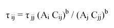 |
(A5.1) |
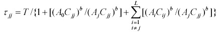 |
(A5.2) |
Choice of base lakes
We will assume that people allocate themselves among different lakes according to a discrete choice model. See Anderson et al. (1992) for this theory and a detailed explanation of its historical origins in psychology and economics, as well as different rationales for the underlying assumptions that lead to the following probability structure. In general, these models assume that utility of choice j is random and is of the form
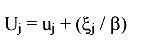 |
(A5.3) |
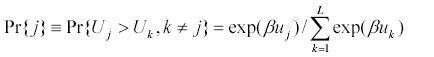 |
(A5.4) |
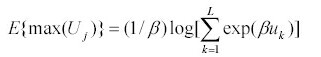 |
(A5.5) |
In the context of our model, the number of people based at lake k in time step t is
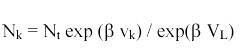 |
(A5.6) |
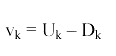 |
(A5.7) |
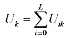 |
(A5.8) |
 |
(A5.9) |
The measure of inclusive value is a natural one and nests the deterministic case where one simply chooses the most valuable alternative, i.e., the case β =  .
.
Fishing effort
The fishing effort on lake i is simply the sum over all base lakes of the number of agents multiplied by the time spent fishing lake i by a representative agent
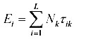 |
(A5.10) |
We assume that the differential equation for influx or efflux of users to or from the lake district is
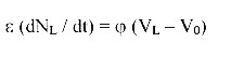 |
(A5.11) |
 converts the difference in value between vacation at the lake district and an alternate vacation into units of people per unit time.
The solution of this differential equation from time t to time t + 1 is
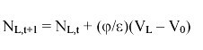 |
(A5.12) |
FOR MULTILAKE CASE
The utility for a representative angler based on lake j is
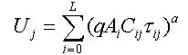 |
(A6.1) |
where the summation goes from zero, representing nonangling activity, to L, for lakes numbered 1 through L.
On a given lake j, effort
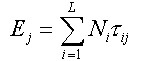 |
(A6.2) |
where the summation is over i for lakes 1 through L. Ni is the number of anglers based on lake i. This effort level is entered into the trophic triangle model to calculate an equilibrium fish stock Aj*. The optimal distributions of fishing time for all anglers on all lakes, τij**, is found by numerically maximizing the sum of Uj over all lakes, subject to the values of A*j determined by the τij*.
The policies pij that evoke optimal management can be included in the utility function for a representative angler
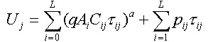 |
(A6.3) |
The first summation is over i from 0 to L. The second summation, which covers only policies that affect fishing, is over i from 1 to L. The optimal time allocation is found using a LaGrange multiplier
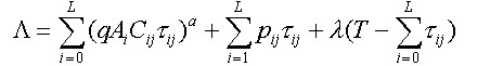 |
(A6.4) |
The third summation is over i from 0 to L, reflecting the entire time budget including time spent in activities other than angling. The LaGrange multiplier λ and the policies pij are found by differentiating Eq. A2.4 with respect to the τij, setting the resulting expressions equal to zero, and inserting the values of the τij**:
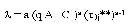 |
(A6.5) |
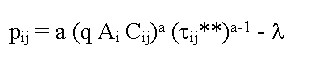 |
(A6.6) |
ONE-SIZE-FITS-ALL POLICY
This appendix describes the method for calculating the one-size-fits-all policies used in A System of Two Lakes in the text to calculate the results in Tables 2 and 3. For a representative person based on lake j, utility is
|
Uj = (q A0 Cjj
0j)a + (q Aj Cjj jj)a + (q Ai Cij ij)a
|
(A7.1) |
The overall time constraint is T = τ0j + τF and the total fishing time τF = τjj + τij. Ai and Aj are set to the equilibrium values of the ecosystem model (Appendix 3) that corresponds to total effort on lake j by anglers based on the two lakes, as in Appendix 6. A0 is the fish equivalent of the alternative nonfishing activities available to a person based on lake j. Values of τF, τ11, and τ22 that maximize U1 + U2 are calculated by numerical optimization methods. Then the optimal policy p is calculated by maximizing the LaGrangian
|
Λ = (q A0 Cjj t0j)a + (q Aj Cjj jj)a + (q Ai Cij ij)a - p F + (T - F - 0j)
|
(A7.2) |
which, using the optimal time allocation for lake 1, leads to
 = a (q A0 C11)a 01a-1 = a (q A0 C11)a 01a-1 |
(A7.3) |
and
|
p = a (q A2 C21)a (
F - 11)a-1 - |
(A7.4) |
This appendix presents some details of the simulations.
Table 8.1. Parameter values used in simulations. See Appendix 1 for parameter definitions. In the table below, v is the vulnerability coefficient for juvenile fishes, not value.
| Parameter | Tables 1–3 |
Fig. 4 |
Figs. 5–6 |
Figs. 7–16 |
|||||||||||||||||||||||||
| β | Not used |
Not used |
Not used |
0.1 (base case) |
|||||||||||||||||||||||||
| a | 0.5 |
0.5 |
0.5 |
0.5 |
|||||||||||||||||||||||||
| cF | 1.1 |
1.1 |
1.1 |
1.1 |
|||||||||||||||||||||||||
| cJ | 0.8 |
0.8 |
0.8 |
0.8 |
|||||||||||||||||||||||||
| f | 0.8 |
0.8 |
0.8 |
0.8 |
|||||||||||||||||||||||||
| g | 1.3 |
1.3 |
1.3 |
1.3 |
|||||||||||||||||||||||||
| h | 10 |
10 |
Varied |
Function of N (see below) |
|||||||||||||||||||||||||
| m | 0.001 |
0.001 |
0.001 |
0.001 |
|||||||||||||||||||||||||
| q | See caption |
0.01 |
0.008 |
0.0001 |
|||||||||||||||||||||||||
| s | 0.75 |
0.75 |
0.75 |
0.75 |
|||||||||||||||||||||||||
| S | Not used |
100 |
5 |
Not used |
|||||||||||||||||||||||||
| v | 10 |
10 |
10 |
10 |
|||||||||||||||||||||||||
Calculation of refuging parameter from resident population
In the landscape simulations (Figs. 7), the refuging parameter hi for a lake I was a function of the number of residents on the lake Ni, as follows
|
hi = (hmax + hmin) - [hmax Ni2 / (hhalf2 + Ni2)]
| (A8.1) |
where hmax = 100, hmin = 0.1, and hhalf = 1000.
Matlab 5.3 code for spatial simulations (Figs. 7–14)
This program was run in Matlab 5.3 to generate the spatial simulations. The different patterns in the simulations were generated by varying β, q, and the travel costs. The code for the comanaged simulations is similar, except that total harvest was not allowed to exceed the escapement level (A = 300).
% Global declarations
clear global
global q fA rF cJA cJF cFA vuln hide surv F0 Effi Ao

% Number of time steps to simulate
tstep=30;
% Number of lakes to simulate
L=25;  % Number of lakes
Lp=21; % Number of lakes with private shoreline (L-Lp = # wilderness lakes)
unit=ones(L,1);

% Define economic parameters
alpha=0.5;  % exponent for production function
balpha=alpha./(1-alpha);  % b(alpha) in pseudocode
T=4;  % Total fishing time available to each person
beta=0.1;  % Intensity parameter for choosing a base lake for vacation
psi=5;  % Rate parameter that converts vacation value to flux of vacationers
epsilon=1;  % Speed-tuning parameter for flux of vacationers
pmove=0.2;  % Proportion of cottage owners who can move each time step
travcost=1;  % Cost to travel one unit of distance for a vacation
addwild=1;  % Additional travel cost for wilderness lake
Cmax=4;  % Maximum inverse cost value for calculating inverse cost matrix
Chalfsat=4;  % Half-saturation parameter for calculating inverse cost matrix
V0vec=50.*ones(tstep,1);  % Value of a vacation at an alternate site

% Define fish parameters
q=1e-4;  % Catchability
fA=0.8;  % Fecundity of adults
rF=1.3;  % r for forage fish
cJA=1.e-3;  % Density-dependent (cannibalism) mortality rate of juveniles
cJF=0.8;  % Consumption rate of juveniles by forage fish
cFA=1.1;  % Consumption rate of forage fish by adults
vuln=10;  % Vulnerability coefficient
% Parameters for computing hiding coefficient from nij (see hidetest.m)
hidemin=0.1;  % Minimum hiding coefficient when housing density is high
hidemax=100; % Maximum hiding coefficient with no houses on lake
hidehalf=1000; % Half-saturation housing density for hiding coef
hideq=2;  % Exponent -- controls slope of hiding function near hidehalf
% End hiding coefficient parameters
surv=0.75;  % Overwinter survivorship
F0=300;  % Density of forage fish at the beginning of each year

% Alternative activity on base lakes
valt=(0.5.*Chalfsat).*(0.25./cJA);  % Half the travel avg X fraction of max fish
valtb=exp(balpha.*log(valt));
valtbvec=valtb.*unit;

% Define vector of lakes and the cost parameters
Lloc=linspace(1,L,L)';  % Vector of lake locations
Lloc(Lp+1:L,1)=Lloc(Lp+1:L,1)+(addwild.*ones(L-Lp,1));  % Additional travel cost of wilderness lakes
Dis2City=L.*unit;  % Distance to population center
Dvec= Dis2City + Lloc;  % Distances from population center
for j=1:L,
   Dmat(:,j)= abs(Lloc(j,1).*unit - Lloc); % Matrix of interlake distances
   C(:,j)=Cmax.*unit./(Chalfsat.*unit + Dmat(:,j));  % inverse costs of travel among lakes
end;

% Set up initial fish vector
Amax=1000;
Amin=50;
% Set up initial fish vector using a hyperbola
halfish=3;  % Half-saturation point along lake gradient
findex=linspace(0,L-1,L)';
A0=Amin.*unit + ( (Amax-Amin).*findex./(halfish.*unit + findex) );

%Set up initial housing vector (see initest.m)
% Use only the lakes that can have private cottages
N0=2e4;  % People on entire landscape
intpil=zeros(L,1);
agg=0.25;  % Degree of aggregation (slope of exponential distrib)
lindex=linspace(0,Lp-1,Lp)';
constant=(exp(agg) - 1)./(exp(agg.*(Lp)) - 1);  % Normalizing constant
for i=0:Lp-1,
   numterm=exp(agg.*Lp - agg.*i - agg);
   intpil(i+1,1)=numterm.*constant;
end;
N0vec=N0.*intpil;

% Set up output matrices
N1vec=zeros(tstep+1,1);
N1vec(1,1)=N0;
VLvec=zeros(tstep,1);
Nimat=zeros(L,tstep+1);
Nimat(:,1)=N0vec;
vkmat=zeros(L,tstep);
Effimat=zeros(L,tstep+1);
Aimat=zeros(L,tstep+1);
Aimat(:,1)=A0;  % Set initial fish distribution

% Update over one time step
for time=1:tstep,

   % Calculate time spent on base lakes
   Amat=A0*unit';  % Columns are # fish in each lake; each column is the same
   ACmat=Amat.*C;
   ACb=exp(balpha.*log(ACmat));  % (Ai * Cij)^b
   % Vector of times spent on base lakes
   tjj = T./( unit + (valtbvec./diag(ACb)) + (sum(ACb)…
		-diag(ACb)')'./diag(ACb));
   % Matrix of times spent on any lake i from base lake j
   tij=(tjj*unit').*ACb./(diag(ACb)*unit');

   % Calculate utility of fishing lake i for a person based on lake j
   Uij = exp(alpha.*log(Amat.*C.*tij));

   % Calculate total utility of fishing from a base lake j
   Uj = sum(Uij);

   % Calculate inclusive value of a vacation at the lake district
   vj=Uj'- (Dvec.*travcost);
   % Inclusive value of vacation
   VL=(1./beta).*log(sum(exp(beta.*vj(1:Lp,1)))); % sum over cottaged lakes

   % Update the number of people vacationing in the lake district
   V0=V0vec(time,1);
   N1=N0 + (psi./epsilon).*(VL-V0);

   % Update number of people based on lake j, for lakes with cottages only
   NewN1j=(N1./(exp(beta.*VL))).*exp(beta.*vj(1:Lp,1));
   NewN1j(Lp+1:L,1)=zeros(L-Lp,1);  % Zeroes for wilderness lakes
   N1j=(1-pmove).*Nimat(:,time) + (pmove.*NewN1j);

   % Calculate fish mortality on lake i
   Effvec=tij'*N1j;
   Mi=q.*A0.*Effvec;

   % Update hide parameter as a function of N1j
   n1jq=exp(hideq.*log(N1j+0.1.*unit));
	hidehalfq=exp(hideq.*log(hidehalf));
   hidevec=hidemax.*unit + hidemin.*unit - ...
      (hidemax.*n1jq./(hidehalfq.*unit + n1jq));

   % Integration parameters
   nint=10;  % Number of intervals for integration
	tspan=[0 1];
   for i=1:L,  % Loop over lakes to integrate fish eqs over one season
      hide=hidevec(i,1); % Habitat is a function of n1j
      Effi = Effvec(i,1);
      Ao=surv.*A0(i,1);
		Y0=fA.*surv.*A0(i,1);
   	[tode,Y1]=RKfix('FishFunk2',tspan,Y0,nint);
      nout=length(tode);
      A1(i,1)= Ao.*exp(-q.*Effi) + Y1(nout,1);
   end; % End loop over lakes

   % Update state variables
   N0=N1;
   A0=A1;

   % Fill output matrices
   N1vec(time+1,1)=N1;
   VLvec(time,1)=VL;
   Nimat(:,time+1)=N1j;
   vkmat(:,time)=vj;
   Aimat(:,time+1)=A0;
   Effimat(:,time+1)=Effvec;

end;  % End of loop over time

function yprime=FishFunk2(t,Y)

% Function for fish population dynamics using direct integration
% for Adults and Forage Fish
% SRC 25 Jan 03

global q fA rF cJA cJF cFA vuln hide uexp surv F0 Effi Ao

At = Ao.*exp(-q.*Effi.*t);
cFAqE=cFA./(q.*Effi);
Ft = F0.*exp(rF.*t - cFAqE.*Ao + cFAqE.*At);

dJdt = -(cJA.*Y.*At) ...
   - cJF.*vuln.*Ft.*Y./(vuln + hide + cJF.*Ft);

yprime = dJdt;
Address of Correspondent:
Stephen R. Carpenter
Center for Limnology
University of Wisconsin-Madison
Madison, Wisconsin 53706 USA
Phone: (608) 262-8690
Fax: (608) 265-2340
srcarpen@wisc.edu
![]()