Supplemental results
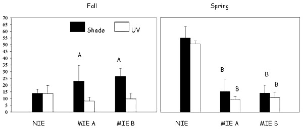
During the October 1998 experiment, realized production of offspring for Amphiascus tenuiremis was significantly less in UV-exposed contaminated sediment in the two Murrell Inlet estuary sites, i.e., MIE A and MIE B, than for the same sediment without UV exposure (P < 0.001; Fig. A1.1). In the May 1999 experiment, realized reproductive success in UV-exposed contaminated sediment was significantly lower than UV-exposed clean sediment from the North Inlet control site (P < 0.0001). Meanwhile, realized offspring production in the UV-shaded contaminated sediment from MIE A and MIE B was also significantly lower than it was in the UV-shaded clean sediment from the North Inlet (P < 0.0001). In the October 1998 experiment, reproductive output by the copepods was greater for those in UV-shaded contaminated sediment in Murrell Inlet than it was for those in UV-shaded clean sediment in the North Inlet. Realized offspring production in the clean North Inlet sediment was more than three times greater in the spring than it was in the fall. Sediment contamination, presence of UV, and season were all significant predictors of A. tenuiremis reproductive success in both October 1998 and May 1999 (ANOVA, P < 0.05).
Figure A1.1. Adult Amphiascus tenuiremis realized offspring production in the fall (October 1998) and spring (May 1999) toxicity experiments. ‘A’ indicates offspring production is significantly higher for copepods in UV-shaded contaminated sediment than for copepods in the same sediment exposed to UV. ‘B’ indicates offspring production is significantly reduced for contaminated sediments in the Murells Inlet Estuary sites (MIE A and MIE B) relative to clean sediments from the North Inlet Estuary (NIE) under the same light exposure. Error bars represent one sample standard deviation.
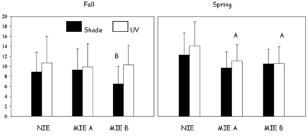
In the October 1998 experiment, average A. tenuiremis clutch size in UV-exposed contaminated sediment at MIE B was significantly higher than the same sediment without UV exposure (P = 0.0001; Fig. A1.2). UV-exposed contaminated sediment from both MIE A and MIE B in the May 1999 experiment had significantly lower clutch sizes than UV-exposed sediment from the control site (P < 0.0001). No significant clutch-size effects were observed for sediments not exposed to UV from any of the sites during the May 1999 experiment. Sediment contamination and presence of UV were significant predictors of egg clutch size in both bioassays (ANOVA, P < 0.05).
Figure A1.2. Adult Amphiascus tenuiremis clutch size in the fall (October 1998) and spring (May 1999) toxicity experiments. ‘A’ indicates clutch size is significantly higher for copepods in UV-shaded contaminated sediment than for copepods in the same sediment exposed to UV. ‘B’ indicates clutch size is significantly reduced for the Murells Inlet Estuary sites (MIE A and MIE B) relative to the North Inlet Esturay (NIE) under the same light exposure. Error bars represent one sample standard deviation.
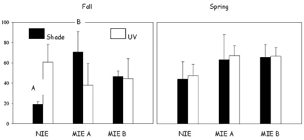
In October 1998, the percentage of females that were gravid at the end of the test was significantly reduced by co-exposure to UV and PAH-contaminated sediment at MIE A relative to the same sediment without UV exposure (P = 0.0035; Fig. A1.3). The percentage of gravid females was also significantly higher for UV-shaded contaminated sediment at MIE A than for the UV-shaded sediment from the control site (P < 0.0001). UV exposure of control site sediments had a significant positive effect on the percentage of egg-carrying females when compared to UV-shaded sediment from the same site (P = 0.0004). Contamination and UV exposure were significant predictors of the percentage of females that were gravid at the end of both tests (ANOVA, P < 0.05).
Figure A1.3. Percentage of Amphiascus tenuiremis gravid females in the October 1998 (fall) and May 1999 (spring) toxicity test. ‘A’ indicates the percentage of gravid females is significantly reduced in UV-shaded sediment relative to the same sediment exposed to UV. ‘B’ indicates the percentage of gravid females is significantly higher in UV-shaded sediment than in the same sediment exposed to UV. MIE = Murrells Inlet estuary; NIE = North Inlet estuary. Error bars represent one sample standard deviation.
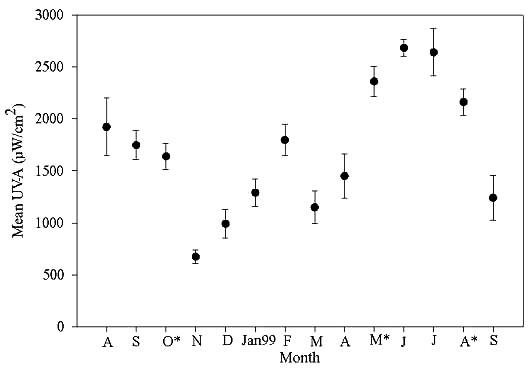
Results of semivariance analyses are provided in Table 2 in the main text. Average UV intensities varied throughout the year (Fig. A1.4), a result that reflects the findings of Literathy et al. (1990). The minimum initial UV intensity occurred in November 1998, when average initial UV was 674.96 ± 67.8 μW/cm2 (mean ± SE). Other low months were the winter months of December 1998 and January 1999, with levels of 993 ± 136 μW/cm2 and 1291 ± 133 μW/cm2, respectively. September 1999 was also relatively low when compared with other months, at 1241 ± 217 μW/cm2. In contrast, surface UV measured in June of 1999 was as high as 2682.60 ± 80.5 μW/cm2. Other summer months, i.e., May, July, and August, were consistently high as well, with UV-A levels of 2360 ± 147 μW/cm2, 2639 ± 225 μW/cm2, and 2161 ± 124 μW/cm2, respectively. The results of the UV sampling were not surprising, because lower UV levels were observed during winter months, and the highest levels were measured in the spring and summer, as observed by Literathy et al. (1990). Complete UV samplings of all sites occurred during October 1998, May 1999, and August 1999. These months represent three unique seasons and were therefore used in the grid modeling.
Figure A1.4. Average initial intensity of ultraviolet light in the UV-A range by month. Error bars represent one sample standard deviation.
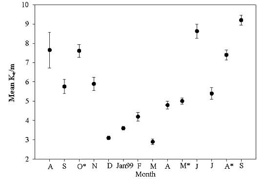
Extinction coefficients varied considerably during the year (Fig. A1.5). Trends in extinction levels increased in the fall of 1998, dropped off considerably during winter and spring months, and rose again in the summer and fall of 1999. The highest extinction coefficients, i.e., lowest UV levels penetrating the water column, were observed during the summer and fall months of August, September, and October of 1998 and June, August, and September of 1999, with Ke values of 7.65 ± 0.923/m (mean ± SE), 5.76 ± 0.37/m, 7.61 ± 0.33/m, 8.63 ± 0.36/m, 7.41 ± 0.26/m, and 9.16 ± 0.26/m, respectively. The lowest extinction levels occurred in December 1998 and January, February, and March of 1999, with Ke values of 3.11 ± 0.09/m, 3.55 ± 0.1/m, 4.22 ± 0.22/m, and 2.92 ± 0.14/m, respectively. Average extinction coefficients at MIE A and MIE B ranged from a minimum of 3.75 ± 0.15/m to a maximum 12.75 ± 1.47/m (Fig. 13 in main text). The lowest average Ke was observed close to the mouth of the inlet, and the highest was calculated at a site in the extreme northern portion of the estuary, adjacent to the landward side of the estuary. However, it is important to note that Ke values at the different sites varied greatly throughout the year. For example, at one site, Ke was 6.34 ± 0.37/m, but had a range of 2.03–22.35/m. This type of variation occurred at one-third of all the sites measured.
Figure A1.5. Average extinction coefficients for all months. Error bars represent one sample standard deviation. An asterisk (*) indicates sampling at all 30 sites.
Extinction coefficients varied considerably over space and time. The highest values and lowest UV penetration were concentrated in the shallow inland areas of the estuary, particularly in the extreme northern and southern portions of the inlet. Lower values and the highest UV penetration were focused near the mouth of the inlet and in nearby deeper portions of MIE. Silt-clay content may help to explain distribution of Ke. The areas characterized by higher silt-clay, and thus higher carbon, contents were also found to have higher extinction coefficients. Lower silt-clay, and thus higher sand, content was observed in the deeper parts of the inlet, close to the mouth. This suggests that sediments with high silt and clay contents, which have a tendency to become resuspended by activities such as boating and wave action, will scatter incident light, resulting in less UV penetration through the water column, as in Ireland et al. (1996). Because of a decrease in observed anthropogenic activities during the winter months, resuspension of particulate matter is less likely, resulting in lower extinction coefficients and higher UV penetration to the creek bed.
When silt-clay content was used to predict Ke in a linear regression model, this variable was found to be significant (P < 0.0001) in the regression. These results suggest that Ke may be explained and/or predicted in terms of silt-clay content. It may be possible to develop a model to calculate Ke if the silt-clay content of bottom sediments is known by measuring incident UV intensity. It was anticipated that, even though the highest levels of PAHs were found in the northern, urbanized portion of the estuary, the high UV extinction occurring there may effectively minimize any potential for hazard, thus providing a protective effect in these more contaminated areas.
Seasonal trends in extinction coefficients may be explained, in part, by phytoplankton cycles in the water column. Phytoplankton population densities are often highest during the month of September in Murrells Inlet (D. L. White, personal communication) and in other estuarine areas (Smayda 1957, Patten et al. 1963, Mallin et al. 1991). Peaks in phytoplankton populations have also been observed during the month of June (Carpenter 1971). These peaks in phytoplankton in the water column coincide with peaks in extinction levels observed during the current study. UV-A and UV-B seawater extinction coefficients (see Methods) were 4.88 ± 0.3/m and 6.9 ± 1.1/m (mean ± SE), respectively, at the sediment-water interface. Using these coefficients in the Kirk (1994) equation, actual A. tenuiremis UV-A and UV-B exposures were 581.17 ± 5 μW/cm2and 76.91 ± 2.25 μW/cm2, respectively. These values are approximately 32% of fall (October 1998) field exposures. Spring mean sediment-water interface UVA and UV-B exposures were 583.06 ± 4.83 μW/cm2 and 77.62 ± 1.12 μW/cm2. Laboratory test values are approximately 25% of spring field exposures based upon May 1999 field measurements. Water quality parameters for the fall and spring toxicity tests were within acceptable limits (American Society for Testing and Materials 1980).
The spring toxicity tests indicated that co-exposure of A. tenuiremis to UV and PAH-contaminated sediments caused significant mortality (30% on average). These results are consistent with studies using Rhepoxynius abronius (Swartz et al. 1990, Boese et al. 1998), Lumbriculus variegates (Ankley et al. 1994, Monson et al. 1995), Hyallela azteca (Ankley et al. 1994), and Daphnia magna (Holst and Giesy 1989). However, in the fall, co-exposure of A. tenuiremis to UV and PAH-contaminated sediments did not appear to cause significant lethal toxicity at the UV and somewhat higher total PAH levels tested here. These findings are consistent with a study involving the midge Chironomus tentans (Ankley et al. 1994), H. azteca, and L. variegates and similar predominant PAH congeners, i.e., fluoranthene, pyrene, and chrysene. When exposed for 10 days to PAH-contaminated sediments with UV, C. tentans survival was unaffected, but H. azteca and L. variegates suffered more than 60% mortality.
Increased copepod reproductive toxicity occurred during the October 1998 experiment in UV-exposed contaminated sediments relative to non-UV exposures of the same sediments. Similarly, reproductive toxicity was seen in the branchiopod Daphnia magna when exposed to low levels of UV (31–117 μW/cm2 UVA) and 190–880 μg/L anthracene solutions (Holst and Giesy 1989). Reproductive toxicity also occurred during the May 1999 experiment, but these results were similar for contaminated sediments exposed to UV or not exposed to UV. This indicates that reproductive toxicity was not enhanced by UV exposure. In May 1999, realized offspring production in control sediments exposed to UV and not exposed to UV was more than three times greater than that measured in October 1998. UV-related clutch size effects were not consistent across experiments. In the October 1998 experiment, UV exposure actually enhanced egg clutch size at one contaminated sediment site. In May 1999, UV-exposed contaminated sediments resulted in significantly smaller clutch sizes than the UV-exposed control sediments, suggesting a UV effect. Significant differences in clutch size were not observed among contaminated sediments that were not exposed to UV, indicating that toxicity tests conducted in the absence of UV light may not measure potential reproductive toxicity in the environment.
UV exposure had an effect at both the control and the PAH-contaminated sites during the October 1998 experiment. The percentage of egg-carrying females was significantly greater in the UV-exposed control sediment, whereas the UV-exposed contaminated sediment showed significant increased toxicity relative to the same sediment without UV exposure. These results suggest that UV alone is not toxic to A. tenuiremis. Rather, it appears to enhance reproduction. However, when UV exposure is combined with PAH contamination, enhanced reproductive toxicity can occur.
A model to predict the 10-d LC50 (lethal concentration, 50%) phototoxicity of specific PAH congeners was developed by Swartz et al. (1990). This model generally characterizes the PAHs with lower solubilities as the most phototoxic. According to the model, among the most phototoxic PAH congeners, arranged from greatest to least phototoxic potential, are anthracene (the most phototoxic), chrysene (extremely phototoxic), benzo(a)pyrene, and benzo(b)fluoranthene. All of these congeners were detected in Murrells Inlet sediments, with chrysene and benzo(b)fluoranthene common in our test sediments. Copepod reproduction in all PAH-contaminated sediment treatments was low, whereas chrysene and benzo(b)fluoranthene were consistently high (92.9–219 ng/g) relative to other congeners. The present study may extend the predictability of the Swartz model to copepod reproductive endpoints.
Supplemental conclusions
Without limiting exposure to specific contaminants, i.e., spiking sediment with known levels of specific chemicals, it is impossible to attribute toxicity to a particular class of contaminants. However, because contaminated sediments in the field are composed of a complex mixture of chemicals nearly impossible to duplicate in the laboratory, it is necessary to use field sediments in toxicity tests. Newsted and Giesy (1987) developed a method for predicting the photoinduced toxicity of PAH mixtures to another zooplankton, Daphnia magna, based on PAH structure and absorption properties as well as organism transmittance. A similar study could be designed for our organism using the PAHs comprising our total PAH level. Another predictive model developed by Swartz et al. (1990) explained the toxicity of field PAH mixtures by considering factors such as toxic units, PAH structure, additivity, and the 10-d LC50 determination. Developing a study such as this one using Murrells Inlet sediments and incorporating the UV effect would help predict photoinduced toxicity in Murrells Inlet.
The previously noted C. tentans survival after UV exposure may be attributed to a more efficient system for dealing with oxidative stress caused by photoactivated PAHs or an exoskeleton that reduces UV penetration to assimilated PAHs. These possibilities should be explored with respect to A. tenuiremis. It would be beneficial to conduct a study co-exposing A. tenuiremis to UV and water-only PAH solutions to investigate whether these fine sediments refract UV. The tendency of A. tenuiremis to burrow may result in the reduction of UV-activated bioaccumulated PAHs. Thus, organism ecology and structure should be considered when evaluating PAH phototoxicity. In addition, the potentially different mixture effects on mortality should be explored further. Presently, neither total PAH concentration nor individual concentration differences can easily explain the lack of consistency in fall and spring PAH lethality.
In the future, the hazard model will be improved by additional laboratory experiments using a range of sites in the Murrells Inlet estuary with varying UV intensities. By obtaining results from a variety of sites, a more complete model could be generated with a broader range of PAH levels. It would also be beneficial to investigate the length of co-exposure to PAHs and UV as a potential hazard factor. In addition, replicate UV measurements at sites, including determination of UV-B, would more effectively characterize UV intensities during the course of the day, potentially supporting a more realistic hazard model.