Biodiversity, Urban Areas, and Agriculture: Locating Priority Ecoregions for Conservation

Taylor Ricketts¹ and Marc Imhoff²

• Abstract
• Introduction
• Methods
  • Ecoregions and species data
  • Land use data
  • Analyses
• Results
• Discussion
• Responses to this Article
• Acknowledgments
• Literature Cited

Urbanization and agriculture are two of the most important threats to biodiversity worldwide. The intensities of these land-use phenomena, however, as well as levels of biodiversity itself, differ widely among regions. Thus, there is a need to develop a quick but rigorous method of identifying where high levels of human threats and biodiversity coincide. These areas are clear priorities for biodiversity conservation. In this study, we combine distribution data for eight major plant and animal taxa (comprising over 20,000 species) with remotely sensed measures of urban and agricultural land use to assess conservation priorities among 76 terrestrial ecoregions in North America. We combine the species data into overall indices of richness and endemism. We then plot each of these indices against the percent cover of urban and agricultural land in each ecoregion, resulting in four separate comparisons. For each comparison, ecoregions that fall above the 66th quantile on both axes are identified as priorities for conservation. These analyses yield four “priority sets” of 6–16 ecoregions (8–21% of the total number) where high levels of biodiversity and human land use coincide. These ecoregions tend to be concentrated in the southeastern United States, California, and, to a lesser extent, the Atlantic coast, southern Texas, and the U.S. Midwest. Importantly, several ecoregions are members of more than one priority set and two ecoregions are members of all four sets. Across all 76 ecoregions, urban cover is positively correlated with both species richness and endemism. Conservation efforts in densely populated areas therefore may be equally important (if not more so) as preserving remote parks in relatively pristine regions.

KEY WORDS: North America, agriculture, biodiversity, conservation, conservation priorities, ecoregions, endemism, human land use, species richness, threats to biodiversity, urbanization.

Published: October 14, 2003

As illustrated by the variety of papers in this special issue, urbanization is one of the most important threats to biodiversity worldwide. Urban areas may threaten ecosystems through direct habitat conversion (e.g., Clergeau et al. 1998, Blair 1999, McKinney 2002) and through various indirect effects of dense human population such as resource use, habitat fragmentation, waste generation, and freshwater cooption (e.g., Mikusinski and Angelstam 1998). Agriculture is another, perhaps even greater, global threat to biodiversity. Similarly to urbanization, agriculture presents both direct problems of habitat conversion and indirect effects of chemical pollution and disturbance of water and nutrient cycles (Pimentel et al. 1992, Vitousek et al. 1997).

Although urbanization and agriculture certainly are global phenomena, their magnitudes differ widely among regions, nor is biodiversity distributed evenly across continents or the globe; hotspots of high species richness and endemism occur, where ecosystem disruption would be especially threatening to global biodiversity (Reid 1998). Therefore, as human population and consumption levels continue to increase, there is a need to develop a quick but rigorous method of identifying where high levels of human threats and biodiversity coincide. These areas are clear priorities for biodiversity conservation, where conservation efforts are most urgent or will do the most good (Ricketts et al. 1999b).

Recently, there have been several efforts to assess geographic priorities for conservation at broad scales. At the global scale, Myers et al. (2000) identified 25 “hotspots,” biogeographic regions where high levels of plant diversity and human threats coincide. Sisk et al. (1994) combined data on mammal and butterfly distributions with information on human demographics and deforestation to identify 18 priority countries worldwide. At a continental scale, Ricketts et al. (1999b) combined quantitative (i.e., species distributions) and qualitative (i.e., expert assessment) data on both biodiversity value and human threats to assess priorities among North American terrestrial ecoregions. Additionally, the U.S. Gap Analysis Program (Scott et al. 1993) has combined species distributions and land management designations to identify underrepresented vegetation types in U.S. protected areas.

These and similar efforts are certainly useful (in fact, several conservation organizations have used their results to prioritize conservation activities), but many have suffered from three key limitations. First, several studies base their analyses on political units (e.g., countries, provinces, counties), because human demographic and species occurrence data are often reported for these boundaries, and because most legal and regulatory systems are based on political units (Sisk et al. 1994, Dobson et al. 1997). However, ecological processes, species ranges, and even anthropogenic threats (e.g., type of agriculture or grazing regimes) typically follow biogeographic rather than political boundaries. Analyses based on political units therefore risk both overlooking important ecosystems within a state or county and hampering assessment of ecosystems that span political borders (Hanks 2000).

Second, these studies often base their analyses on only one or a few groups of species (e.g., Scott et al. 1993, Sisk et al. 1994). This is because consistent distribution data are typically available for only a small number of taxa (e.g., birds, mammals). Authors are thus forced to assume that these taxa serve as informative indicators of overall biodiversity, an assumption that been increasingly challenged (Weaver 1995, Flather et al. 1997, Ricketts et al. 1999a, 2002).

Third, many assessments depend on subjective information, typically in the form of expert opinion, to measure threats to biodiversity (Olson and Dinerstein 1998, Ricketts et al. 1999b, Myers et al. 2000). Quantitative data on human threats have proven difficult to compile over broad scales, especially for nonpolitical geographic units. Faced with these data limitations, relying on expert opinion is a logical choice, but it inevitably results in somewhat subjective and nonrepeatable analyses.

In this study, we combine several recent data sets that relieve some of these limitations and allow us to quantitatively assess conservation priorities among ecological units in North America. We base our analyses on the terrestrial ecoregions of the United States and Canada (Ricketts et al. 1999b). We compare biodiversity among these ecoregions using species distribution data compiled for > 20,000 species in eight taxa, and we measure impacts of urbanization and agriculture using maps derived from remote-sensing imagery. These data sets allow us to analyze patterns of biodiversity, urbanization, and agriculture in a consistent manner across the continent.

We query the combined database to address two main questions. First, where do areas of high biodiversity coincide with areas of intense human land use? These areas are clearly priorities for conservation. Second, how do these priorities differ under different measures of biodiversity (i.e., richness, endemism) and land use (i.e., urban cover, agriculture)? Identifying geographic priorities for conservation in a quantitative manner, and understanding how these priorities depend on the factors considered will help conservationists to allocate resources most efficiently in conserving biodiversity.

Ecoregions and species data

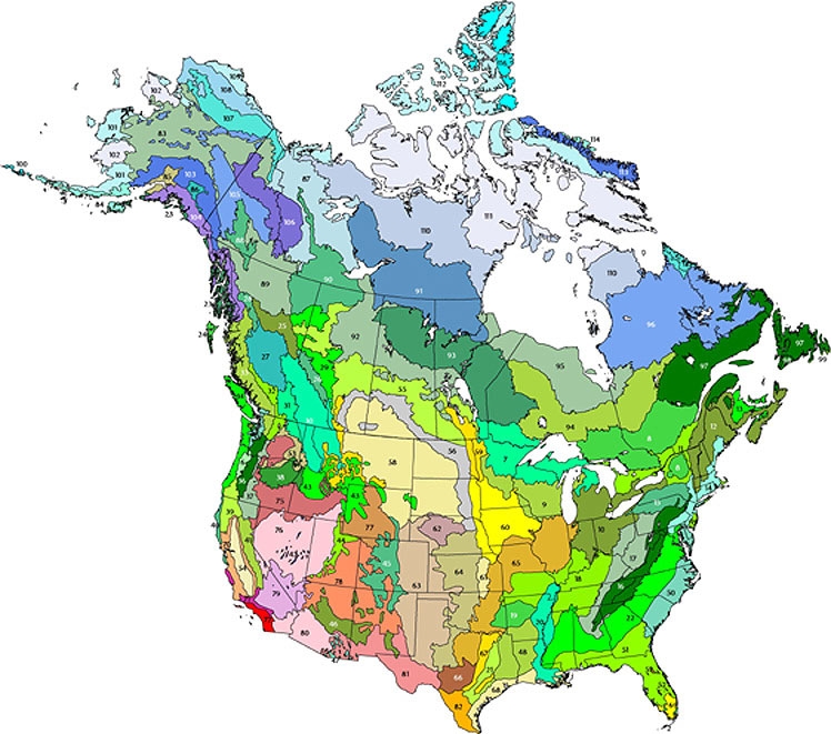
The geographic units that we use for these analyses are the 110 ecoregions of the continental United States and Canada (Fig. 1). These ecoregions were first developed by Ricketts et al. (1999b), and are based largely on three established ecoregion mapping projects (ESWG 1995, Gallant et al. 1995, Omernik 1995). Ecoregions are defined as relatively coarse biogeographic divisions of a landscape that delineate areas with broadly similar environmental conditions and natural communities. Because of the complexity with which environmental and ecological factors vary across a landscape, ecoregion boundaries are necessarily approximate and represent areas of transition rather than sharp divisions.

Fig. 1. Map of the terrestrial ecoregions of the United States and Canada. Numbers on the map correspond to those in Table 1.

For these ecoregions, Ricketts et al. (1999b) compiled published and unpublished data on the distributions of > 20,000 species in eight taxa: birds, mammals, butterflies, amphibians, reptiles, land snails, tiger beetles, and vascular plants. For six taxa, published range maps were compared to the ecoregion map and each species was recorded as present, endemic, or absent in every ecoregion. A species was counted as endemic if it either (1) was found in no other ecoregion, including Mexico and other continents or (2) occupied a range totaling <50,000 km² (following Birdlife International’s threshold for range-restricted species; Bibby 1992). Thus, a species with an exceptionally small range that crossed an ecoregion boundary was recorded as endemic in both ecoregions. For two taxa (vascular plants and land snails), scientists with unpublished databases were consulted to provide richness and endemism estimates for each ecoregion. For all taxa, only native species were included.

Land use data

We used two remotely sensed data sets to measure urban and agricultural land use. For urban cover, we used a map of city lights for North America developed by Imhoff et al. (1997b). This data set is based on nighttime satellite imagery originally designed to map moonlit cloud cover, and it has a spatial resolution of 2.7 km. Imhoff et al. (1997b) use these data to map urbanized areas on the earth’s surface, based on the stability of pixel illumination through time. They recognize three classes of urban cover, calibrated with census data to index human population density: “urban,” with an average of 1064 persons/km²; “peri-urban,” with an average of 100 persons/km²; and “non-urban,” with an average of 14 persons/km². These data thus indicate not only the amount of land directly transformed by urbanization, but also the local human population density and hence the various indirect impacts of human activity on ecosystems (e.g., pollution, other “dark” forms of land use change). For these analyses, we lumped the “urban” and “peri-urban” areas together to create one measure of urbanized land (Fig. 2a).

Fig. 2. Overlay maps of terrestrial ecoregions with (a) urban areas (in red) and (b) agricultural land use (in orange). In both panels, northern hatched areas were excluded from analyses (see Methods).

For agriculture, we used the U.S. Geological Survey’s (USGS) North America Seasonal Land Cover map (Loveland et al. 2000). This map is derived from a time series of satellite images (AVHRR) taken from April 1992 to March 1993 at 1-km resolution. We used the USGS Land Use Land Cover classification of the data (Anderson et al. 1976), which recognizes 24 land classes, five of which are agricultural: “Dryland cropland and pasture,” “Irrigated cropland and pasture,” “Mixed Dryland/Irrigated Cropland and Pasture,” “Cropland/Grassland Mosaic,” and “Cropland/Woodland mosaic.” For these analyses, we lumped these five categories to create one measure of agricultural land cover (Fig. 2b).

It is important to emphasize that these two remotely sensed data sets are independent of political (or any other) geographic units and thus are easily applied to ecoregions or other biologically meaningful geographic units (Imhoff et al. 1997a). In addition, the data are of relatively constant quality across broad regions, instead of relying on county or state records of uneven quality. Because our data for urban cover are less reliable and uncalibrated in higher latitudes due to aurora interference, here we exclude northern areas (corresponding to taiga and tundra biomes) and limit our analyses to the 76 remaining ecoregions (Fig. 2).

Analyses

From the ecoregion database of species presence/absence, we calculated the number of species and the number of endemic species of each taxon in every ecoregion. We then developed indices that integrate data from all eight taxa into overall measures of species richness and endemism. These indices, which combine data from such varied taxa, are likely to be more informative indicators of overall biodiversity than any one taxon alone (Ricketts et al. 1999a).

We defined the richness index as

[1]

where R_i is the richness of taxon i in the ecoregion, and T_i is the total number of species of taxon i in the database. This index (modified from Sisk (1994) and used by Ricketts et al. (1999a)) normalizes the richness of each taxon by the number of North American species in that taxon and then averages those fractions across all eight taxa. It therefore weights taxa evenly, preventing speciose taxa (e.g., vascular plants) from dominating measures of overall richness. This index was normally distributed (Shapiro-Wilk test, W = 0.961, P > 0.05, n = 76), but increased significantly with ecoregion area (Fig. 3a). We controlled for this common effect of area (Rosenzweig 1995) by using the residuals of this regression (Fig. 3a) in all analyses (Sokal and Rohlf 1995).

Fig. 3. Richness and endemism indices vs. ecoregion area: (a) richness (linear regression, r 2 = 0.24, P <0.0001); (b) endemism (nonsignificant).

We defined the endemism index as

[2]

where E_i is the number of endemic species of taxon i in the ecoregion, and R_i is as previously defined. This index computes, for each taxon, the fraction of species in an ecoregion that is endemic there, and then averages these fractions across all eight taxa. This proportional measure of endemism is more meaningful in this context than a simple count of endemic species or other popular measures (e.g., Kershaw et al. 1995), because the latter two are expected to increase with increasing species richness, whereas our index is independent of richness. Endemism was not significantly related to ecoregion area (Fig. 3b). To improve normality, we arcsine-transformed and then log-transformed the endemism index before analysis.

We measured threats as the areal fraction of each ecoregion converted to either urbanized land or agriculture. Both of these measures were arcsine-transformed and then log-transformed to improve normality for analysis.

To identify ecoregions of concern, we plotted the richness and endemism indices against the measures of urbanization and agriculture and identified, for each of the four plots, the ecoregions that fell above the 66th quantile (i.e., in the upper third) on both axes (see Fig. 4c for illustration). Finally, we used the Jaccard index (Jongman et al. 1995) to quantify overlap among these four sets of priority ecoregions.

Fig. 4. Levels of richness and endemism vs. human land use: (a) richness vs. urbanization, (b) richness vs. agriculture, (c) endemism vs. urbanization, and (d) endemism vs. agriculture. To illustrate our analytical approach, 66th quantile lines for identifying priorities are shown in panel (c), and ecoregions above both quantiles are represented by filled circles in all panels. Note the positive relationships between richness and urbanization (r2 = 0.31, P < 0.0001) and between richness and agriculture (r2 = 0.12, P < 0.005), but the lack of such relationships with endemism (both nonsignificant).

Ecoregions vary widely in their levels of both biodiversity and human threats (Table 1). Upon plotting the two diversity indices against the two measures of threat, we find that the richness index is positively related to both urbanization and, to a lesser degree, agriculture (Fig. 4a, b). No such relationship exists between the endemism index and either threat measure (Fig. 4c, d).

Table 1. Richness and endemism indices for each ecoregion, as well as percent cover of urban and agricultural land uses, and membership in priority sets a. Map numbers correspond to those in Fig. 1. Map no.      Ecoregion name Richness index Endemism index Urban cover (%) Agric. cover (%) Richness sets b Endemism    setsc   2 South Florida Rocklands 0.139 0.086 60.1 21.9 urban urban   6 Willamette Valley Forests 0.112 0.026 41.3 33.7   7 Western Great Lakes Forests 0.163 0.012   7.5 31.8   8 Eastern Forest/Boreal Transition 0.153 0.003   5.6   4.1   9 Upper Midwest Forest/Savanna Transition Zone 0.172 0.005 21.2 91.0 10 Southern Great Lakes Forests 0.203 0.010 30.5 76.9 11 Eastern Great Lakes Lowland Forests 0.164 0.002 29.6 40.0 12 New England/Acadian Forests 0.165 0.013 12.2   5.7 13 Gulf of St. Lawrence Lowland Forests 0.101 0.000 23.8 18.4 14 Northeastern Coastal Forests 0.204 0.014 49.0 13.5 urban 15 Allegheny Highlands Forests 0.167 0.007 10.9   2.5 16 Appalachian/Blue Ridge Forests 0.264 0.104 20.5   8.0 urban urban 17 Appalachian Mixed Mesophytic Forests 0.261 0.070 17.3   5.7 urban urban 18 Central U.S. Hardwood Forests 0.250 0.051 17.9 19.5 urban urban 19 Ozark Mountain Forests 0.183 0.049 10.1   5.6 20 Mississippi Lowland Forests 0.191 0.007 18.2 72.9 both 21 East Central Texas Forests 0.191 0.021 12.2 85.6 agric. 22 Southeastern Mixed Forests 0.267 0.057 20.9 16.6 urban urban 23 Northern Pacific Coastal Forests 0.068 0.006   1.5   0.1 24 Queen Charlotte Islands 0.056 0.003   0.4   0.3 25 Northern British Columbia Mountain Forests 0.081 0.000   1.1   0.0 26 Alberta Mountain Forests 0.090 0.000   1.9   0.1 27 Fraser Plateau and Basin Complex 0.095 0.000   3.2   0.4 28 Northern Transitional Alpine Forests 0.075 0.000   0.3   0.0 29 Alberta/British Columbia Foothills Forests 0.094 0.000   9.0   5.5 30 North Central Rockies Forests 0.146 0.042   3.8   1.6 31 Okanogan Dry Forests 0.135 0.023 10.6   3.1 32 Cascade Mountains Leeward Forests 0.106 0.002   2.4   1.5 33 British Columbia Mainland Coastal Forests 0.124 0.003   1.6   0.5 34 Central Pacific Coastal Forests 0.134 0.072   7.1   0.5 35 Puget Lowland Forests 0.111 0.024 47.8   3.8 36 Central and Southern Cascades Forests 0.129 0.061   2.2   0.4 37 Eastern Cascades Forests 0.131 0.004   3.9   5.9 38 Blue Mountains Forests 0.124 0.039   1.9   3.6 39 Klamath-Siskiyou Forests 0.155 0.107   5.9   5.1 40 Northern California Coastal Forests 0.141 0.143 14.6   0.5 41 Sierra Nevada Forests 0.158 0.143   5.3   0.4 42 Great Basin Montane Forests 0.099 0.062   0.8   0.7 43 South Central Rockies Forests 0.133 0.014   2.1   4.0 44 Wasatch and Uinta Montane Forests 0.135 0.018   6.7   2.6 45 Colorado Rockies Forests 0.157 0.014   4.9   0.5 46 Arizona Mountains Forests 0.180 0.074   4.0   0.4 47 Madrean Sky Islands Montane Forests 0.163 0.145   2.2   0.3 48 Piney Woods Forests 0.194 0.011 14.6 18.3 49 Atlantic Coastal Pine Barrens 0.143 0.014 53.9 54.8 both 50 Middle Atlantic Coastal Forests 0.225 0.024 23.6 49.1 both 51 Southeastern Conifer Forests 0.257 0.108 22.3 52.9 both both 52 Florida Sand Pine Scrub 0.139 0.122 49.1 72.7 both both 53 Palouse Grasslands 0.131 0.040   8.3 24.1 54 California Central Valley Grasslands 0.101 0.053 27.0 30.1 both 55 Canadian Aspen Forest and Parklands 0.132 0.000 10.4 71.2 56 Northern Mixed Grasslands 0.164 0.000   7.8 85.8 57 Montana Valley and Foothill Grasslands 0.132 0.010   9.8 26.6 58 Northwestern Mixed Grasslands 0.173 0.007   4.1 43.7 59 Northern Tall Grasslands 0.147 0.004 12.4 93.3 60 Central Tall Grasslands 0.182 0.004 14.5 95.9 61 Flint Hills Tall Grasslands 0.163 0.005   7.0 22.4 62 Nebraska Sand Hills Mixed Grasslands 0.120 0.063   2.2 27.0 agric. 63 Western Short Grasslands 0.232 0.034   7.8 16.4 64 Central and Southern Mixed Grasslands 0.202 0.004 10.1 53.8 65 Central Forest/Grassland Transition Zone 0.256 0.020 17.6 54.9 both 66 Edwards Plateau Savannas 0.187 0.038   8.0 57.1 agric. 67 Texas Blackland Prairies 0.209 0.033 27.2 55.8 both 68 Western Gulf Coastal Grasslands 0.254 0.035 26.8 65.2 both 69 Everglades 0.150 0.066 21.5 40.0 both 70 California Interior Chaparral and Woodlands 0.167 0.158 21.1   2.3 urban 71 California Montane Chaparral and Woodlands 0.157 0.114 15.9   2.1 urban urban 72 California Coastal Sage and Chaparral 0.169 0.157 59.0   0.3 urban urban 75 Snake/Columbia Shrub Steppe 0.153 0.024   6.8 11.8 76 Great Basin Shrub Steppe 0.169 0.066   4.2   1.0 77 Wyoming Basin Shrub Steppe 0.141 0.008   5.2   1.3 78 Colorado Plateau Shrublands 0.239 0.026   5.3   0.8 79 Mojave Desert 0.172 0.165   8.3   0.2 80 Sonoran Desert 0.202 0.139 12.0   3.9 81 Chihuahuan Deserts 0.280 0.095   5.6   0.4 82 Tamaulipan Mezquital 0.192 0.057 12.9 49.7 agric. agric. Meand 0.162 0.043 14.4 23.4 1 SD 0.051 0.047 14.3 28.6      a This table reports raw (untransformed) values. For regression and quantile analyses that follow, data are transformed as described in Methods.      b Ecoregions that rank in the top third for both richness index and for measures of urbanization, agriculture, or both.      c Ecoregions that rank in the top third for both endemism index and for measures of urbanization, agriculture, or both.      d A simple arithmetic mean, not weighted by ecoregion area.

Comparing richness and urbanization yields 16 ecoregions that fall above the 66th quantile on both axes (Figs. 4 and 5, Table 1). The ecoregions in this “priority set” contain both extraordinary species richness and high levels of urbanization. For richness and agriculture, 11 priority ecoregions are similarly identified. Comparing endemism and urbanization yields a priority set of 12 ecoregions. Finally, using endemism and agriculture, six priority ecoregions are identified.

Fig. 5. Maps of priority sets (i.e., ecoregions in the top 66th quantile of biodiversity and land use indices). (a) Richness index vs. urbanization (blue), agriculture (yellow), or both (blue and yellow stripes). (b) Endemism index vs. urbanization (blue), agriculture (yellow), or both (blue and yellow stripes). In both panels, northern hatched areas were excluded from analyses (see Methods).

A key issue is the degree to which these four priority sets overlap. Jaccard indices indicate the highest overlap between the richness/urbanization and endemism/ urbanization sets (Table 2). Indeed, these two sets share nine ecoregions out of 16 and 12, respectively. Overlap is also high between the richness/urbanization and richness/agriculture sets (Table 2); these two sets share eight ecoregions out of 16 and 11, respectively.

Table 2. Jaccard similarity coefficients among sets of priority ecoregions.     Richness         Endemism     Urbanization Agriculture Urbanization Agriculture Richness Urbanization 1 Agriculture 0.42 1 Endemism Urbanization 0.47 0.10 1 Agriculture 0.10 0.21 0.29 1

We found that the distribution of both biodiversity and human threats is extremely heterogeneous in the United States and Canada. For example, some ecoregions contain > 25% of North American species (averaging over the eight taxa considered), whereas other ecoregions contain < 6% (Table 1). Similarly, urbanization varied from < 0.5% to > 60%. This heterogeneity affirms the importance of establishing clear conservation priorities, because some areas are much more threatened or diverse than others.

Of the 76 ecoregions considered, our analyses identified four “priority sets” of 6–16 ecoregions (8–21% of total number) where high levels of biodiversity and human land use coincide (Fig. 5). These ecoregions tend to be concentrated in the southeastern United States, California, and, to a lesser extent, the Atlantic coast, southern Texas, and the U.S. Midwest. Several ecoregions are members of more than one priority set (e.g., the green ecoregions in Fig. 5), and two ecoregions (Southeastern Conifer Forests and Florida Sand Pine Scrub, numbers 51 and 52) are members of all four sets. These ecoregions may be considered of additional concern, as they face multiple sources of habitat destruction and contain both high richness and high endemism.

We were interested to find that species richness was positively correlated with both urbanization and agricultural conversion. It thus appears that humans tend to settle and prosper in the most species-rich areas of the continent. Similar relationships have been reported in Africa (Balmford et al. 2001) and worldwide (Cincotta et al. 2000), suggesting that this may be a general pattern (but see Huston 1993). There are at least two intuitive and interrelated reasons for this result. First, humans tend to prefer climates that also support high species richness. For example, both urbanization and species richness increase significantly toward lower latitudes (data not shown), even with the northernmost ecoregions excluded (see Methods). Second, humans tend to settle in, farm, and build urban centers in highly productive ecosystems (e.g., moist forests, moist grasslands) that also support high levels of biodiversity (Huston 1993, Imhoff 2000, Balmford et al. 2001). Whatever the cause(s), the correlation between species richness and urbanization emphasizes the fact that human activities and biodiversity may be on a collision course. Preserving remote parks in sparsely inhabited regions thus will conserve perhaps only a fraction of the world’s species; we must manage ecosystems simultaneously for both human productivity and biodiversity (Pimentel et al. 1992, Daily et al. 2001).

As in any analysis of conservation priorities, our results depend on the conservation objective. Here, we target areas with extraordinary levels of both biodiversity and human land use, but several other objectives, with equal justification, exist. For example, the goal for some conservation biologists is to conserve the species assemblage of every ecoregion, regardless of its relative richness or endemism. In this case, priorities would be based mostly on the relative degrees of threat (i.e., land-use intensity) among ecoregions. Our results can support this objective as well, by focusing on the land-use data alone to compare ecoregions (Table 1).

In addition, one could ask whether the ecoregions identified here are necessarily the most valuable investments for conservation. Because of high demand for land use, habitat preservation or restoration is likely to be costly and politically difficult in these ecoregions (Ando et al. 1998). At least for species richness, more cost-effective conservation opportunities may lie in neighboring ecoregions with similar habitat types and communities, but with lower land prices and demand. A similar approach may be to target the positive outliers of the relationship in, for example, Fig. 4a; these points represent ecoregions containing significantly higher species richness than expected, given their level of urbanization. They may therefore represent the most “bang for the buck” in terms of land prices and feasibility of land preservation.

Because opinions differ on approaches and objectives, prioritization exercises should maintain sufficient transparency to allow alternative interpretations and support various conservation goals. Nevertheless, it is important to note that endemic species, by definition, can be conserved only in their ecoregion of occurrence; local extirpation of a narrowly endemic species may result in global extinction. Therefore, ecoregions containing both high endemism and high human threats are among the clearest conservation priorities (Fig. 5b).

Spatial scale is another attribute that affects both the results and utility of any priority analysis. Our analysis is based on relatively large ecoregions and is therefore necessarily coarse. Clearly, species and ecosystems are most directly protected through activities at finer scales, such as habitat and landscape conservation plans, reserve design and establishment, and improved land management. International and regional NGO’s have increasingly developed approaches for coordinating these and other activities to maximize the overall benefit to local populations and communities (Groves et al. 2002, Sanderson et al. 2002, Kambem-Toham et al. 2003). However, these efforts often require large investments of time and resources; they simply cannot be carried out everywhere at once. Simple, coarse-scale analyses such as this one can help to quickly focus these efforts where they have the potential to deliver the most benefit (Noss 1990, Olson and Dinerstein 1998).

At the same time, finer scale analyses and efforts can inform and refine broader priority schemes. For example, although our analyses identify ecoregions in which human land use and endemic species overlap, finer analyses within the ecoregion may reveal that the ranges of those species are, in fact, well protected, with urban and agricultural lands occurring elsewhere in the ecoregion. Ideally, conservation analyses, efforts, and decisions would be made at a range of scales, with insights and results from each informing and strengthening the others (Noss 1990).

One reviewer offered an alternative interpretation of our results: that our priority sets did not represent areas where conflicts can be expected, but rather indicated areas where species are more able to coexist with human activities and land use. Our species data, however, are based on compilations of occurrence records and therefore represent the expected species pool for each ecoregion. Because the data do not reflect recent extirpations or range reductions, regions with high richness should not be interpreted as those that have retained those species despite human activities. Perhaps a more direct method of evaluating the impacts of human activities is to relate human land use to levels of species endangerment among ecoregions (e.g., Dobson et al. 1997). We have begun compiling these data for North America. In the meantime, given the numerous studies showing the negative effects of human land use on biodiversity (e.g., Clergeau et al. 1998, Wilcove et al. 1998, Blair 1999, McKinney 2002), it is reasonable to expect that ecoregions with most intense land use will also experience these effects most intensely.

Comparing our results to those of three similar studies reveals broad agreement on the regions of highest conservation concern, despite differences in approaches and analytical units. First, Stein et al. (2000) found that species richness in the United States is highest in the southwest and southeast regions, a pattern similar to what we report here. Overall richness maps in Stein et al. (2000) appear to emphasize the southwest more than do our results in Fig. 5; this difference is probably because Stein et al. (2000) based their analyses on states, which are larger in the west. In addition, we use an index of richness that weights taxa equally, preventing vascular plants (which are richest in southwestern states) from dominating the measure (see Methods). Second, Noss and Peters (1995) evaluated levels of threat to U.S. ecosystems. In their “Overall Threat Index,” states of “extreme risk” overlap closely with the ecoregions indicated here as members of priority sets. Third, Ricketts et al. (1999b), assessed conservation priorities among these same ecoregions, relying heavily on expert opinion. Of the 23 ecoregions identified here as priorities (Table 1, Fig. 5), 18 (78%) were also placed in the two highest priority classes by Ricketts et al. (1999b).

However, Ricketts et al. (1999b) were able to identify 13 additional priority ecoregions, based on other aspects of biological importance (e.g., globally important migrations) and threat (e.g., grazing) that are difficult to measure in a quantitative, consistent manner across the continent. For example, the Chihuahuan desert (#81) scored the highest in our richness index, but was not included in a priority set because the most important human impact on this ecoregion is grazing (Ricketts et al. 1999b). Similarly, ecoregions in the Pacific Northwest of the United States are left out of priority sets because they are primarily threatened by logging (Ricketts et al. 1999b), which we were not able to measure. These ecoregions serve to illustrate the sensitivity of these analyses to the input data used, and the potential limitations of strictly quantitative approaches.

This study has focused on local impacts of urbanization and agriculture, but it is clear that human activities affect ecosystems in neighboring and even distant ecoregions. For example, New York City consumes resources from farms, cattle ranches, and forests throughout North America and, indeed, the world (Chichilnisky and Heal 1998). Considering the impacts of the city’s urban area and population only within its ecoregion is clearly an oversimplification, and it remains a significant challenge to relate centers of human population to their spatially explicit “ecological footprints” (Wackernagel and Yount 1998). Nevertheless, perhaps the majority of impacts from urbanization and agriculture are felt by local ecosystems. It therefore will continue to be informative and valuable to compare patterns of biodiversity and anthropogenic threats in order to identify broad-scale priorities for conservation.

Responses to this article are invited. If accepted for publication, your response will be hyperlinked to the article. To submit a comment, follow this link. To read comments already accepted, follow this link.

We thank K. Bowen, J.P. Fay, M. Mayfield, J. Schwan, and W. Wettengel for assistance with data management and analyses. C. Allen, C. Boggs, K. M. Carney, J. Hellmann, C. Loucks, and three anonymous reviewers improved the manuscript with their ideas and comments. Support from NASA (NAG5-8563-001 and NAG5-9760-002) and The Summit Foundation is also gratefully acknowledged.

Anderson, J. R., E. E. Hardy, J. T. Roach, and R. E. Witmer. 1976. A land use and land cover classification system for use with remote sensor data. U.S. Geological Survey Professional Paper 964. U.S. Government Printing Office, Washington, D.C., USA.

Ando, A., J. Camm, S. Polasky, and A. Solow. 1998. Species distributions, land values, and efficient conservation. Science 279:2126–2128.

Balmford, A., J. L. Moore, T. Brooks, N. Burgess, L. A. Hansen, P. Williams, and C. Rahbek. 2001. Conservation conflicts across Africa. Science 291:2616–2619.

Bibby, C. J. 1992. Putting biodiversity on the map: priority areas for global conservation. International Council for Bird Preservation (ICBP), Washington, D.C., USA.

Blair, R. B. 1999. Birds and butterflies along an urban gradient: surrogate taxa for assessing biodiversity? Ecological Applications 9:164–170.

Chichilnisky, G., and G. Heal. 1998. Economic returns from the biosphere. Nature 391:629–630.

Cincotta, R. P., J. Wisnewski, and R. Engelman. 2000. Human population in the biodiversity hotspots. Nature (London) 404:990–992.

Clergeau, P., J. P. L. Savard, G. Mennechez, and G. Falardeau. 1998. Bird abundance and diversity along an urban-rural gradient: A comparative study between two cities on different continents. Condor 100:413–425.

Daily, G. C., P. R. Ehrlich, and G. A. Sanchez-Azofeifa. 2001. Countryside biogeography: use of human-dominated habitats by the avifauna of southern Costa Rica. Ecological Applications 11:1–13.

Dobson, A. P., J. P. Rodriguez, W. M. Roberts, and D. S. Wilcove. 1997. Geographic distribution of endangered species in the United States. Science 275:550–553.

ESWG (Ecological Stratification Working Group). 1995. A national ecological framework for Canada. Agriculture and Agri-food Canada, Research Branch, Centre for Land and Biological Resources Research; and Environment Canada, State of the Environment Directorate, Ecozone Analysis Branch, Ottawa/Hull, Ontario, Canada.

Flather, C. H., K. R. Wilson, D. J. Dean, and W. C. McComb. 1997. Identifying gaps in conservation networks: of indicators and uncertainty in geographic-based analyses. Ecological Applications 7:531–542.

Gallant, A. L., E. F. Binnian, J. M. Omernik, and M. B. Shasby. 1995. Ecoregions of Alaska. Professional Paper 1567, U.S. Geological Survey, Washington, D.C., USA.

Groves, C. R., D. B. Jensen, L. L. Valutis, K. H. Redford, M. L. Shaffer, J. M. Scott, J. V. Baumgartner, J. V. Higgins, M. W. Beck, and M. G. Anderson. 2002. Planning for biodiversity conservation: putting conservation science into practice. BioScience 52:499–512.

Hanks, J. 2000. The role of transfrontier conservation areas in southern Africa in the conservation of mammalian biodiversity. Cambridge University Press, Cambridge, UK.

Huston, M. 1993. Biological diversity, soils, and economics. Science 262:1676–1680.

Imhoff, M. L. 2000. The use of multisource satellite and geospatial data to study the effect of urbanization on primary productivity in the United States. Transactions on Geoscience and Remote Sensing 38:2549–2556.

Imhoff, M. L., W. T. Lawrence, C. D. Elvidge, T. Paul, E. Levine, M. V. Privalsky, and V. Brown. 1997a. Using nighttime DMSP-OLS images of city lights to estimate the impact of urban land use on soil resources in the United States. Remote Sensing of Environment 59:105–117.

Imhoff, M. L., W. T. Lawrence, D. C. Stutzer, and C. D. Elvidge. 1997b. A technique for using composite DMSP-OLS "city lights" satellite data to map urban area. Remote Sensing of Environment 61:361–370.

Jongman, R. H. G., C. J. F. ter Braak, and O. F. R. Van Tongeren, editors. 1995. Data analysis in community and landscape ecology. Cambridge University Press, New York, New York, USA.

Kambem-Toham, A., A. W. Adeleke, N. D. Burgess, R. Carroll, J. D'Amico, E. Dinerstein, D. M. Olson, and L. Some. 2003. Forest conservation in the Congo basin. Science 299:346.

Kershaw, M., G. M. Mace, and P. H. Williams. 1995. Threatened status, rarity, and diversity as alternative selection measures for protected areas: a test using afrotropical antelopes. Conservation Biology 9:324–334.

Loveland, T. R., B. C. Reed, J. F. Brown, D. O. Ohlen, J. Zhu, L. Yang, and J. W. Merchant. 2000. Development of a global land cover characteristics database and IGBP DISCover from 1-km AVHRR data. International Journal of Remote Sensing 21:1303–1330.

McKinney, M. L. 2002. Urbanization, biodiversity, and conservation. BioScience 52:883–890.

Mikusinski, G., and P. Angelstam. 1998. Economic geography, forest distribution, and woodpecker diversity in central Europe. Conservation Biology 12:200–208.

Myers, N., R. A. Mittermeier, C. G. Mittermeier, G. A. B. daFonseca, and J. Kent. 2000. Biodiversity hotspots for conservation priorities. Nature 403:853–858.

Noss, R. F. 1990. Indicators for monitoring biodiversity: a hierarchical approach. Conservation Biology 4:355–364.

Noss, R. F., and R. L. Peters. 1995. Endangered ecosystems: A status report on America's vanishing habitat and wildlife. Defenders of Wildlife, Washington, D.C., USA.

Olson, D. M., and E. Dinerstein. 1998. The Global 200: a representation approach to conserving the Earth's most biologically valuable ecoregions. Conservation Biology 12:502–515.

Omernik, J. M. 1995. Level III ecoregions of the continental US.. U.S. Environmental Protection Agency, Washington, D.C., USA.

Pimentel, D., U. Stachow, D. A. Takacs, H. W. Brubaker, A. R. Dumas, J. J. Meaney, J. A. S. Oneil, D. E. Onsi, and D. B. Corzilius. 1992. Conserving biological diversity in agricultural forestry systems: most biological diversity exists in human-managed ecosystems. BioScience 42:354–362.

Reid, W. V. 1998. Biodiversity hotspots. Trends in Ecology and Evolution 13:275–280.

Ricketts, T. H., G. C. Daily, and P. R. Ehrlich. 2002. Does butterfly diversity predict moth diversity? Testing a popular indicator taxon at local scales. Biological Conservation 103:361–370.

Ricketts, T. H., E. Dinerstein, D. M. Olson, and C. Loucks. 1999a. Who's where in North America: patterns of species richness and the utility of indicator taxa for conservation. BioScience 49:369–381.

Ricketts, T. H., E. Dinerstein, D. M. Olson, C. Loucks, W. Eichbaum, K. Kavanagh, P. Hedao, P. Hurley, K. M. Carney, R. Abel, and S. Walters. 1999b. Terrestrial ecoregions of North America: a conservation assessment. Island Press, Washington, D.C., USA.

Rosenzweig, M. L. 1995. Species diversity in space and time. Cambridge University Press, Cambridge, UK.

Sanderson, E. W., K. H. Redford, A. Vedder, P. B. Coppolillo, and S. E. Ward. 2002. A conceptual model for conservation planning based on landscape species requirements. Landscape and urban planning 58:41–56.

Scott, J. M., F. Davis, B. Csuti, R. Noss, B. Butterfield, C. Groves, H. Anderson, S. Caicco, F. D'erchia, T. C. Edwards Jr., J. Ulliman, and R. G. Wright. 1993. Gap analysis: a geographic approach to protection of biological diversity. Wildlife Monographs 123:1–41.

Sisk, T. D., A. E. Launer, K. R. Switky, and P. R. Ehrlich. 1994. Identifying extinction threats: global analyses of the distribution of biodiversity and the expansion of the human enterprise. BioScience 44:592–604.

Sokal, R. R., and F. J. Rohlf. 1995. Biometry. Third edition. W. H. Freeman, New York, New York, USA.

Stein, B. A., L. S. Kutner, G. A. Hammerson, L. L. Master, and L. E. Morse. 2000. State of the states: geographic patterns of diversity, rarity, and endemism. In B. A. Stein, L. S. Kutner, and J. S. Adams, editors. Precious heritage: The status of biodiversity in the United States. Oxford University Press, New York, New York, USA.

Vitousek, P. M., H. A. Mooney, J. Lubchenco, and J. M. Melillo. 1997. Human domination of Earth's ecosystems. Science 277:494–499.

Wackernagel, M., and J. D. Yount. 1998. The ecological footprint: an indicator of progress toward regional sustainability. Environmental Monitoring and Assessment 51:511–529.

Weaver, J. C. 1995. Indicator species and scale of observation. Conservation Biology 9:939–942.

Wilcove, D., D. Rothstein, J. Dubow, A. Phillips, and E. Losos. 1998. Quantifying threats to imperiled species in the United States. BioScience 48:607–615.