|
|
|
Copyright © 1997 by The Resilience Alliance*
van Coller, L. 1997. Automated techniques for the qualitative analysis of ecological models: continuous models. Conservation Ecology [online]1(1): 5. Available from the Internet. URL: http://www.consecol.org/vol1/iss1/art5/
To print the entire article (including any tables, figures, or appendices), use this link to the unified version of the article.
To print separate parts of the article, click in the frame containing that part (text, figure, table, or appendix) before choosing File, Print.
Research Automated Techniques for the Qualitative Analysis of Ecological Models: Continuous Models Lynn van Coller1
Department of Mathematics,University of British Columbia
- Abstract
- Introduction
- Ratio-Dependent Model
- Resilience
- Conclusion
- Acknowledgments
- Responses
- Literature Cited
KEY WORDS: bifurcation; computer analysis; dynamical systems; ecological models; qualitative analysis; ratio-dependent model; XPPAUT.
Caution: If your browser does not handle graphics, the mathematical models and all Greek characters will be unreadable in this online version. Please email the author to obtain a complete hard copy.
Most parameter values in nature are not known with certainty (Hadamard 1952, Frank 1978). It is also well known that different parameter values in a model can give rise to very different dynamics, such as stable equilibrium behavior, oscillatory behavior, or a decline to extinction. However, finding parameter combinations that give rise to these different dynamics is often a matter of trial and error and involves numerous simulations. The dynamical systems software provides an easier and more systematic way to do this.
In this paper, I substantiate this claim by using the software XPPAUT (Ermentrout 1994), which contains an interface to AUTO86 (Doedel 1981), to analyze three continuous ecological models of varying complexity. Appendix 5 contains a list of other packages that have capabilities similar to XPPAUT or AUTO86. In the main body of this paper, I consider only one of these models in detail. This model is a recent example from the controversial area of ratio-dependent modeling. It has three state variables that represent a plant, a herbivore, and a predator. In addition to highlighting some of the limitations of an isocline analysis in this three-dimensional setting, the analysis shows that the model is structurally unstable. Even small perturbations to the ratio-dependent terms alter the dynamics.
Because this paper is intended as an introduction to the application of dynamical systems techniques to ecological models, I include a number of appendices. Appendix 2 introduces some of the ideas and terminology and also provides a glossary of the terms used in the paper and appendices. Those readers unfamiliar with dynamical systems ideas may benefit from a quick reading of this appendix before continuing. A more comprehensive exposition, also specifically written for ecologists, can be found in Yodzis (1989). Another excellent introduction to nonlinear dynamics can be found in Strogatz (1994). Appendix 3 shows how the dynamical systems techniques can be applied to a fairly simple predator-prey model using XPPAUT. I show how I reproduced and improved on Bazykin's analytical results (Bazykin 1974) for the model. This appendix establishes some confidence in the reliability of the computer software.
Appendix 4 discusses the application of the software to a system dynamics model that has 10 state variables and a large number of parameters. Analytical work done by hand and isocline analyses are of little use in such situations. Traditionally, computers have been used to obtain numerical solutions corresponding to a fixed parameter set and to implement sensitivity analyses. In Appendix 4, I show how dynamical systems techniques can be used to increase our understanding of the relationships between different components in the model. In particular, bifurcation diagrams give more information than sensitivity analyses. These diagrams also highlight an incomplete relationship in the model and lead to an improvement in the formulation of the equations. Thus, the packages can help us to formulate more plausible models.
I also discuss the topic of model resilience, a concept introduced by Holling (1973), to parameter and population perturbations.
I also claim that the technique used by Gutierrez et al. (1994) to study the model, namely isocline analysis (for technique and examples, see Edelstein-Keshet 1988), is unsuitable in this three-dimensional setting. This is discussed in detail in section 2.2.4. Although isocline analyses have been employed in many settings and with considerable success (Fitzhugh 1961, Rosenzweig and MacArthur 1963, Gilpin 1974, Hethcote 1976, Ludwig et al. 1978, Fairen and Velarde 1979, Murray 1981), in more complicated, higher dimensional models for which the categorization of variables as slow vs. fast is not possible, their application is limited. (If the state variables in a model vary on different time scales, it is often possible to approximate the system by a two-dimensional model representing either the slow or the fast dynamics. An isocline analysis can then be done using the reduced system.) An isocline analysis allows two variables, at most, to vary simultaneously. This means that, for the current model, one variable is held fixed, resulting in a partly static representation of the dynamics. However, the dynamical systems techniques allow all three state variables to vary simultaneously, thus permitting a more accurate analysis.
2.1 Model Equations
The basic model equations and a description of the parameters can be found in Appendix 1. There are three equations describing the dynamics of a plant, a herbivore, and a predator. In Appendix 1, I describe how I nondimensionalized the equations and introduced a small modification to the ratio-dependent terms. The resulting equations are as follows:
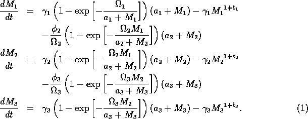
In the next section, I compare results from the original model, (ai = 0) with those from the modified equations (ai = 0.001). I chose this latter value for the ai's because it only affects the isocline configurations (see Appendix 1) at low values of the state variables, which is where the difficulties with the ratio-dependent model are encountered. I also investigate a few other values.
2.2 Model analysis
2.2.1 One-parameter studies
Gutierrez et al. (1994) did a partial qualitative analysis of the original model, but used different techniques (namely, isocline analysis), so it will be informative to compare some of the results. I chose dimensionless parameters with this in mind (see Appendix 1). Because one of the main conclusions in Gutierrez et al. (1994) concerns the relative efficacy of two parasitoids in controlling the cassava mealybug population, I begin by studying two parameters that affect the third trophic level, namely and
and
 . I then discuss some
parameters affecting the herbivore. Only a few examples are included
here. Results, together with possible biological interpretations, are
described in the next section.
. I then discuss some
parameters affecting the herbivore. Only a few examples are included
here. Results, together with possible biological interpretations, are
described in the next section.
2.2.2 Analysis of the predator parameters
The parameter can be thought of as the potential
predator biomass growth rate when prey are abundant, or as the
predator's conversion efficiency in the presence of abundant
prey. Note that the value of
does not affect the isoclines. The
M3 zero isocline is given by
 , and the solution of
this equation is independent of
(see equations
(1). Hence, an
isocline analysis similar to that done in Gutierrez et al. (1994)
would not give any insight into how this parameter influences the
behavior of the system.
, and the solution of
this equation is independent of
(see equations
(1). Hence, an
isocline analysis similar to that done in Gutierrez et al. (1994)
would not give any insight into how this parameter influences the
behavior of the system.
Bifurcation diagrams showing the effects of varying
for both the original
and the modified model are shown in
Fig. 1, with
M1 plotted on the y-axis. These
diagrams were obtained using AUTO through XPPAUT. In both Fig. 1
diagrams, the position of the equilibrium point does not vary with
, supporting the
previous observation that
does not affect the isocline
configuration. However,
does affect the stability of the
system. In both cases, the equilibrium point is unstable for very low
values of (low
predator growth rate) and the stable attractor is a limit cycle for
these values. The original model gives an example of hard loss of
stability (see
Appendix
2) so that, for certain values of
, there are two stable attractors,
a sink and a stable limit cycle (as in
Fig. 11). The
initial values of the state variables determine which final state is
reached. Also, perturbations to the system may cause a rapid change
from one stable attractor to the other if the disturbance is
sufficiently large. For a very small range of
values near the Hopf bifurcation
point HB in Fig. 1a, there are two stable limit cycles. The range of
values is so small, however, that it is not of much biological
significance.
Analysis of the temporal dynamics of the system (using XPPAUT) for
different values of
shows that larger values of
decrease the time
taken to reach equilibrium. Increasing
, the potential growth rate of the
predator, has a stabilizing influence on the system. This seems
biologically plausible, because higher values of
suggest that the predator is better
adapted to controlling its prey. Interestingly, this trait does not
affect any of the equilibrium biomasses. The modified model has a
much smaller range of parameter values over which cycles occur, and
the amplitudes of these cycles are smaller than for the original model
(see Fig. 1). Thus, even though the ai' s
have small values, they appear to have a stabilizing influence on the
dynamics.
, the
availability (or nutritional value) of the herbivore to the predator,
also directly affects the predator. Bifurcation diagrams for the
original and modified models, respectively, are shown in
Fig. 2 and Fig. 3. From these
figures, it can be seen that as
increases, there is a general
increase in the M1 equilibrium value, or
limit cycle maximum. The larger
, the greater the availability of
the herbivore to the predator and the easier it is for the predator to
control the herbivore. Obviously, the lower the herbivore population,
the higher the plant equilibrium. As the M1
equilibrium value approaches the M1 carrying
capacity in the original model, a Hopf bifurcation (see Appendix 2)
occurs at = 0.09
(see Fig. 2). The periodic orbit associated with this Hopf bifurcation
undergoes a number of period-doubling bifurcations (see Appendix 2),
which leads to more complicated cycling behavior. An example of the
temporal dynamics when
 is shown in
Fig. 4. The
minima of the M2 and
M3 cycles, in particular, get very small (on
the order of 10-15, according to XPPAUT's data
window). From a practical viewpoint, these populations would be
considered extinct due to statistical variation, in which case the
plant population would increase to its carrying capacity for these
values of . This
is exactly the case for the modified model (see Fig. 3). Thus, the
upper Hopf bifurcation may be an artifact of ratio-dependent
models. This will be discussed in more detail later.
is shown in
Fig. 4. The
minima of the M2 and
M3 cycles, in particular, get very small (on
the order of 10-15, according to XPPAUT's data
window). From a practical viewpoint, these populations would be
considered extinct due to statistical variation, in which case the
plant population would increase to its carrying capacity for these
values of . This
is exactly the case for the modified model (see Fig. 3). Thus, the
upper Hopf bifurcation may be an artifact of ratio-dependent
models. This will be discussed in more detail later.
These low minima also lead to numerical difficulties, resulting
from the way in which the model is formulated, particularly the
dependence of many of the terms on the ratio
 . These ratios become difficult to
evaluate numerically as Mi approaches zero,
causing the ratio to tend to infinity. XPPAUT fails to calculate zero
isoclines, whereas AUTO often enters an infinite loop if such a
situation arises and may crash. Setting a fairly low total number of
steps for a continuation sometimes allows AUTO to break out of the
loop and signal nonconvergence. Manually stopping a continuation when
one of the state variables gets very close to zero also prevents the
package from crashing. This explains why the limit cycles in Fig. 2
are only calculated up to
. These ratios become difficult to
evaluate numerically as Mi approaches zero,
causing the ratio to tend to infinity. XPPAUT fails to calculate zero
isoclines, whereas AUTO often enters an infinite loop if such a
situation arises and may crash. Setting a fairly low total number of
steps for a continuation sometimes allows AUTO to break out of the
loop and signal nonconvergence. Manually stopping a continuation when
one of the state variables gets very close to zero also prevents the
package from crashing. This explains why the limit cycles in Fig. 2
are only calculated up to
 . Such problems do not occur when
using the modified model.
. Such problems do not occur when
using the modified model.
has a
significant effect on the equilibrium values of the state
variables. This is in agreement with Gutierrez et al. (1994), but the
way in which they arrive at this conclusion is not entirely
correct. Gutierrez et al. (1994) state that a less efficient
parasitoid has a wider C-shaped
M2-isocline. It is true that if
is decreased, the
M2-isocline widens. However, this is
provided that M3 is
constant. If the system is integrated and
M3 is allowed to vary until a new equilibrium
is reached, and the isoclines are plotted with this new equilibrium
M3 value, then the final
M2-isocline may, in fact, have a narrower C
shape than before.
This analysis has shown that the properties of the predator affect the stability of the system as well as the equilibrium magnitudes of the herbivore (directly) and the plant (indirectly). The extent of these effects depends on the properties of both the plant and the herbivore. In the next section, a parameter affecting the herbivore is examined in more detail.
2.2.3 Analysis of a herbivore parameter
Varying  , the
assimilation or conversion efficiency of the herbivore when plants are
abundant, gives the bifurcation diagrams in
Fig. 5. Comparing Fig. 5b with Fig. 3a reveals that they are almost
mirror images. If the mean of the cycle maxima and minima in Fig. 5a
and Fig. 2a is taken, then these two figures are also almost mirror
images. That is, decreasing
has a very similar effect to
increasing . Both
parameters can be thought of as affecting the resistance of the
herbivore to the predator. Decreasing
causes a decline in the condition
of the herbivore, because it cannot convert food as effectively. As a
result, the detrimental effect of the predator on the herbivore is
greater. Increasing
, the availability (nutritional
value) of the herbivore to the predator, achieves the same result but
more directly.
, the
assimilation or conversion efficiency of the herbivore when plants are
abundant, gives the bifurcation diagrams in
Fig. 5. Comparing Fig. 5b with Fig. 3a reveals that they are almost
mirror images. If the mean of the cycle maxima and minima in Fig. 5a
and Fig. 2a is taken, then these two figures are also almost mirror
images. That is, decreasing
has a very similar effect to
increasing . Both
parameters can be thought of as affecting the resistance of the
herbivore to the predator. Decreasing
causes a decline in the condition
of the herbivore, because it cannot convert food as effectively. As a
result, the detrimental effect of the predator on the herbivore is
greater. Increasing
, the availability (nutritional
value) of the herbivore to the predator, achieves the same result but
more directly.
Two-parameter diagrams in
(,
)-space can be generated by
continuing the Hopf bifurcations in Fig. 5 in two parameters. The
results are shown in
Fig. 6. These
diagrams show clearly that decreasing
or increasing
has a similar effect, since the
Hopf bifurcation curves occur roughly along the diagonal that has one
end at the origin. Part of this result could have been predicted from
Gutierrez et al. (1994), because they note that it is the ratio
of and
that determines the
nature of the herbivore isocline. This inverse relationship is thus
expected. However, the one-parameter bifurcation diagrams give us the
additional information that, for certain parameter ranges, limit
cycles are possible.
Some important observations can be made by comparing the Fig. 6
diagrams. First, AUTO could not calculate beyond the point denoted by
MX in Fig. 6a; this problem does not occur in Fig. 6b. A closer
investigation reveals that the equilibrium values for the state
variables are close to zero in the upper left triangle of the
two-parameter space, and this results in numerical problems when using
the original model. Figure 6b gives a more complete picture of the
dynamics. There are two regions that correspond to stable cycles,
whereas stable tritrophic equilibria occur in the other region. Low
values of give
rise to high equilibrium values of M1 and
high values of
give rise to low equilibrium values, an ecologically important
distinction. A comparison of the two Fig. 6 diagrams shows that the
dynamics for the modified model, although very similar to those for
the original model, are more stable in general. That is, the region
corresponding to tritrophic equilibria is larger and the cycles in the
upper half of the two-parameter space are less complex. These claims
are made clearer in
Fig. 7 and Fig. 8.
Figure 7 shows the
(,
)-space for the modified model with
ai =0.002 (i = 1,2,3). The
region of stable equilibria is even larger than in Fig. 6b, resulting
in smaller regions of cycles. The presence of the ai
's seems to have a stabilizing effect on the dynamics of the
system. Figure 8 shows time plots corresponding to points marked with
*'s in the left-hand section of the upper region of cycles in
Figs. 6a, b, and Fig. 7. The left-hand portion of this region is where the
values of M2 and M3
are low and, hence, where the nonzero ai 's
have most effect. Clearly, nonzero ai 's
reduce the complexity of the cycles (even for very small values), and
increasing their values also reduces the cycle
amplitude. Additionally, the cycles for the original model
(ai =0, i = 1,2,3) undergo
long periods of extremely low values, which is unrealistic from an
ecological viewpoint.
2.2.4 The role played by the isocline configurations
From their isocline analysis, Gutierrez et al. (1994) concluded that the parasitoid Epidinocarsis lopezi could control the cassava mealybug, whereas E. diversicornis could not. However, with three state variables all having similar time scales, these deductions are not as straightforward as they may seem. First, the equilibrium isocline configuration in the M1M2(M2M3) phase plane depends on the value of M3(M1) as well as the parameter values. Thus, noting how an isocline changes as a parameter is varied does not give a complete picture. Second, it is impossible to tell from the qualitative structure of the isoclines which intersection point in the M1M2 plane corresponds to a tritrophic equilibrium. Figure 9 shows three possibilities. Two of these (Fig. 9b and c) appear in Gutierrez et al. (1994), who assumed, incorrectly, that the equilibrium point in Fig. 9b was unstable.
Even if the exact position of the equilibrium point is known, it is
impossible to tell, from the qualitative structure of the isoclines,
whether this point is stable or unstable and whether or not limit
cycles occur. For example, although altering the parameter
has no effect on the
isoclines, low values of
give rise to unstable fixed points
and stable limit cycles, and high values give rise to a stable
equilibrium (see Fig. 1). Thus, numerical computation is needed to
determine the exact location as well as the local stability of an
equilibrium point for the current model.
In general, it is the proximity of the tritrophic equilibrium point to the peaks of the M1 and M2 isoclines in the M1M2 and M2M3 planes, respectively, that is important for determining the robustness of model behavior with respect to parameter perturbations. If the equilibrium point is close to one of these peaks, then a small parameter perturbation may change the qualitative structure of the isoclines and, hence, the dynamics. However, to obtain this information, the exact equilibrium isocline configuration for a given set of parameter values needs to be known.
By inference, these criticisms have all noted that if the exact positions of the isoclines and the tritrophic equilibrium were known in both phase planes, then we could obtain a fair amount of information from them. Using XPPAUT, this is possible. In particular, the effects of introducing nonzero values for the ai's can be studied. Figure 10 shows the results obtained using the reference parameter set for model 1 (Eq. A1.1) of Appendix 1 with ai = 0, ai = 0.001, and ai = 0.005 (i = 1, 2, 3).
A comparison of Fig. 10a and b demonstrates that introducing the ai's prevents the M1 and M2 isoclines from passing through the origin. Hence, the equilibrium values for the state variables do not approach zero as rapidly as for the original model, and the modified model is more robust to parameter variations in this region of low biomasses. Increasing the ai's from 0.001 to 0.005 reduces the humped shape of the M1 and M2 isoclines. The result is an even more robust model. In fact, when ai = 0.005 (i = 1, 2, 3), no regions of cycling behavior are encountered when the various parameters are altered. Because values of 0.005 are still small, this suggests that the model is structurally unstable and, hence, predictions from ratio-dependent models should be treated with caution.
2.3 Discussion The preceding analysis has shown how XPPAUT and AUTO can be used to study the effects of various parameters on the behavior of the ratio-dependent model of Gutierrez et al. (1994). Regions of stable equilibria, sustained oscillations, and multiple equilibria were located in this study. The limitations of an isocline analysis in this three-dimensional setting were also discussed, thus supporting the need for new techniques such as the dynamical systems ones.
The ease with which models may be studied using XPPAUT allowed the simultaneous study of the original model and a modified one. I concluded that the original model is structurally unstable, because a small perturbation to the ratio-dependent terms has a significant effect on the dynamics. This supports the argument that ratio-dependent models exhibit pathological behavior and are not valid near the axes (see the background information for ratio-dependent models in Appendix 1). Thus, they cannot be used to study extinction or situations in which one of the state variables attains low values. However, the model by Gutierrez et al. (1994) that has been analyzed is a biological control model whose aim is to suggest what kind of predator can keep herbivore numbers low.
This paper aims to show the usefulness of dynamical systems computer packages and to indicate the ease with which they may be used to gain insights into the behavior of a model and, thus, concentrates on these points. However, the arguments should not be taken out of context. My claim is not that the packages provide a comprehensive way in which to study ecological models. Instead, they should be seen as aids to be used in conjunction with other methods of analysis. Also, these packages do have their limitations. They can only be used to study systems of ordinary differential equations where all the functions are continuous (although simple step functions can often be approximated by continuous functions, as is done in Appendix 4 for the sheep-hyrax-lynx model). Other types of models require different methods of analysis. The packages also require an initial set of parameter values to be chosen. Thus, other techniques are required for theoretical studies that aim to find the exact parameter relationships giving rise to different types of behavior. However, numerical studies can be useful for indicating the relationships that do exist, and thus can provide direction for theoretical studies.
Wollkind et al. (1988) use the latter definition to examine the resilience of their model system for predator-prey mite interactions to changes in food quality of prey for conversion into predator births. This resilience depends on the range of parameter values that give rise to a certain type of qualitative behavior. The wider this range, the greater the system�s resilience to perturbations of the relevant parameter, provided the parameter is not too near the range endpoints.
Collings and Wollkind (1990) discuss the resilience of various stable phenomena in their model, which exhibits metastability. In this case, the resilience is in terms of the magnitude of population (rather than parameter) perturbations that the system can withstand. If a stable phenomenon has a small domain of attraction (see Appendix 2), then small changes to the populations can lead to dramatic changes in system behavior. Such a system is not resilient.
Both of these studies used bifurcation diagrams to obtain results. Thus, bifurcation diagrams can characterize the resilience of a model system to both parameter and population perturbations. In the sheep-hyrax-lynx model in Appendix 4, the stable equilibrium behavior predominates for wide ranges of the parameter values that were considered. Because there was only a single equilibrium point, the system is resilient to both population perturbations and perturbations in the sheep female culling normal (SFCN), provided SFCN is within the desirable range of values and the initial population values are reasonable.
The ratio-dependent model is less resilient, in that parameter
perturbations can push the system from stable equilibrium behavior
into oscillatory behavior and vice versa. However, Fig. 6 shows that
the regions of stable and oscillatory behavior in
 space are fairly large. Hence, for
parameter combinations that are well within these regions, the system
is resilient to small perturbations in
and
.
space are fairly large. Hence, for
parameter combinations that are well within these regions, the system
is resilient to small perturbations in
and
.
The results obtained were compared with those from traditional approaches. AUTO improved on some approximations that Bazykin (1974) made in his analytical study of a predator-prey model. In the sheep-hyrax-lynx model (Swart and Hearne 1989), the bifurcation diagrams gave more information than a traditional sensitivity analysis. This highlighted a relationship that had been omitted from the model. Thus, the dynamical systems techniques can be helpful in constructing better models.
For the ratio-dependent model (Gutierrez et al. 1994), XPPAUT allowed two variations of the model to be studied simultaneously. The resulting conclusion was that the original model is structurally unstable, due to its ratio-dependent terms. The dynamical systems techniques also highlighted the limitations of an isocline analysis in a three-dimensional setting.
In addition, the bifurcation diagrams can be used to characterize the resilience of models to both parameter and population perturbations.
The most important point of this paper is that dynamical systems software was used to arrive at these conclusions. A complete understanding of the underlying mathematical techniques is not required to obtain useful information about the behavior of a model. The software also allows complicated models to be analyzed in greater depth than was previously possible. It is also possible to study discrete models, the topic of a second paper.
None of the models in this paper has a seasonal component. Seasonality plays an important role in the dynamics of many natural systems; thus, studies of models that include such components would be of interest. A few such studies using dynamical systems techniques have been done (e.g., Rinaldi et al. 1993, Gragnani and Rinaldi 1995), but the bifurcation structure is more complicated than that discussed in this paper and requires a continuation package that can handle higher codimension bifurcations, such as LOCBIF (Khibnik et al. 1993; see Appendix 5). Because this paper is intended to introduce the application of dynamical systems techniques to ecological models, I have not included one of these more complex examples.
Responses to this article are invited. If accepted for publication, your response will be hyperlinked to the article. To submit a comment, follow this link. To read comments already accepted, follow this link.
- Abrams, P.A. 1994. The fallacies of
"ratio-dependent'' predation. Ecology 75(6): 1842-1850.
- Akçakaya, H.R., R. Arditi, and L.R. Ginzburg. 1995. Ratio-dependent predation: an abstraction that works. Ecology 76(3): 995-1004.
- Allgower, E.L., and K. Georg. 1992. Continuation and path following. Acta Numerica 1-64.
- Arditi, R., and H. Saïah. 1992. Empirical evidence of the role of heterogeneity in ratio-dependent consumption. Ecology 73(5):1544-1551.
- Arnold, V.I. 1983. Geometrical methods in the theory of ordinary differential equations. Springer-Verlag, New York, New York, USA.
- Aronson, D.G., M.A. Chory, G.R. Hall, and R.P. McGehee. 1982. Bifurcations from an invariant circle for two-parameter families of maps of the plane: a computer-assisted study. Communications in Mathematical Physics 83: 303-354.
- Back, A., J. Guckenheimer, M. Myers, F. Wicklin, and P. Worfolk. 1992. dstool: computer-assisted exploration of dynamical systems. Notices of the American Mathematical Society 39: 303-309.
- Bazykin, A.D. 1974. Volterra's system and the Michaelis-Menten equation. Pages 103-142 in V.A. Ratner, editor. Problems in mathematical genetics. U.S.S.R. Academy of Science, Novosibirsk, U.S.S.R.
- Beddington, J.R., C.A. Free, and J.H. Lawton. 1975. Dynamic complexity in predator-prey models framed in difference equations. Nature 255: 58-60.
- Beddington, J.R., C.A. Free, and J.H. Lawton. 1976. Concepts of stability and resilience in predator-prey models. Journal of Animal Ecology 45: 791-816.
- Berlinski, D. 1976. On systems analysis: an essay concerning the limitations of some mathematical methods in the social, political, and biological sciences. Massachusetts Institute of Technology Press, Cambridge, Massachusetts, USA.
- Berryman, A.A. 1992. The origins and evolution of predator-prey theory. Ecology 73(5): 1530-1535.
- Brylinski, M. 1972. Steady-state sensitivity analysis of energy flow in a marine ecosystem Pages xxx-xxx in B.C. Patten, editor. Systems analysis and simulation in ecology, II. Academic Press, New York, New York, USA.
- Collings, J.B., and D.J. Wollkind. 1990. A global analysis of a temperature-dependent model system for a mite predator-prey interaction. SIAM Journal of Applied Mathematics 50(5): 1348-1372.
- Collings, J.B., D.J. Wollkind, and M.E. Moody. 1990. Outbreaks and oscillations in a temperature-dependent model for a mite predator-prey interaction. Theoretical Population Biology 38: 159-191.
- Deuflhard, P., B. Fiedler, and P. Kunkel. 1987. Efficient numerical pathfollowing beyond critical points. SIAM Journal of Numerical Analysis 24: 912-927.
- Doedel, E.J. 1981. AUTO: a program for the automatic bifurcation analysis of autonomous systems. Congressus Numerantium 30: 265-284.
- Dowden, P.B., H.A. Jaynes, and V.M. Carolin. 1953. The role of birds in a spruce budworm outbreak in Maine. Journal of Economic Entomology 46: 307-312.
- Edelstein-Keshet, L. 1988. Mathematical models in biology. Random House, New York, New York, USA.
- Ermentrout, G.B. 1995. XPPAUT 1.63: the differential equations tool.
- Fairen, V., and M.G. Velarde. 1979. Time-periodic oscillations in a model for respiratory process of a bacterial culture. Journal of Mathematical Biology 8: 147-157.
- Fitzhugh, R. 1961. Impulses and physiological states in theoretical models of nerve membrane. Biophysical Journal 1: 445-466.
- Forrester, J.W.1961. Industrial dynamics. Massachusetts Institute of Technology Press, Cambridge, Massachusetts, USA.
- Frank, P.M. 1978. Introduction to system sensitivity theory. Academic Press, New York, New York, USA.
- Freedman, H.I., and R.M. Mathsen. 1993. Persistence in predator-prey systems with ratio-dependent predator influence. Bulletin of Mathematical Biology 55(4): 817-827.
- Gerald, C.F., and P.O. Wheatley. 1989. Applied numerical analysis. Addison-Wesley, Reading, Massachusetts, USA.
- Gilpin, M.E. 1974. A model of the predator-prey relationship. Theoretical Population Biology 5: 333-344.
- Ginzburg, L.R., and H.R. Akçakaya. 1992. Consequences of ratio-dependent predation for steady-state properties of ecosystems. Ecology 73(5): 1536-1543.
- Gleeson, S.K. 1994. Density dependence is better than ratio dependence. Ecology 75(6): 1834-1835.
- Gragnani, A., and S. Rinaldi. 1995. A universal bifurcation diagram for seasonally perturbed predator-prey models. Bulletin of Mathematical Biology 57(5): 701-712.
- Guckenheimer, J., and P. Holmes. 1983. Nonlinear oscillations, dynamical systems, and bifurcation of vector fields. Springer-Verlag, New York, New York, USA.
- Gutierrez, A.P. 1992. Physiological basis of ratio-dependent predator-prey theory: the metabolic pool model as a paradigm. Ecology 73(5): 1552-1563.
- Gutierrez, A.P., N.J. Mills, S.J. Schreiber, and C.K. Ellis. 1994. A physiologically based tritrophic perspective on bottom up-top down regulation of populations. Ecology 75: 2227-2242.
- Hadamard, J. 1952. Lectures on Cauchy's problem in linear partial differential equations. Dover, New York, New York, USA.
- Hale, J.K., and H. Kogak. 1989. Differential and difference equations through computer experiments. Springer-Verlag, New York, New York, USA.
- Hanski, I. 1991. The functional response of predators: worries about scale. Trends in Ecology and Evolution 6(5): 141-142.
- Hearne, J.W. 1987. An approach to resolving the parameter sensitivity problem in system dynamics methodology. Applied Mathematical Modelling 11: 315-318.
- Hethcote, H.W. 1976. Qualitative analyses of communicable disease models. Mathematical Biosciences 28: 335-356.
- Holling, C.S. 1965. The functional response of predators to prey density and its role in mimicry and population regulation. Memoirs of the Entomological Society of Canada 45: 1-60.
- ______ . 1973. Resilience and stability of ecological systems. Annual Review of Ecology and Systematics 4: 1-23.
- Hultquist, P.F. 1988. Numerical methods for engineers and computer scientists. Benjamin Cummings, Menlo Park, California, USA.
- Jeffers, J.N.R. 1978. An introduction to systems analysis with ecological applications. University Park Press, Baltimore, Maryland, USA.
- Kaas-Petersen, C. 1989. PATH: user's guide. University of Leeds, Leeds, UK.
- Khibnik, A., Y. Kuznetsov, V. Levitin, and E. Nikolaev. 1993. Continuation techniques and interactive software for bifurcation analysis of ordinary differential equations and iterated maps. Physica D 62: 360-371.
- Kowal, N.E. 1971. A rationale for modeling dynamic ecological systems. Pages xxx-xxx in B.C. Patten, editor. Systems analysis and simulation in ecology, I. Academic Press, New York, New York, USA.
- Ludwig, D., D.D. Jones, and C.S. Holling. 1978. Qualitative analysis of insect outbreak systems: the spruce budworm and forest. Journal of Animal Ecology 47: 315-332.
- Lundberg, P., and J.M. Fryxell. 1995. Expected population density vs. productivity in ratio-dependent and prey-dependent models. American Naturalist 146(1): 153-161.
- MacDonald, N. 1978. Time lags in biological models. Springer-Verlag, Berlin, Germany.
- ______ . 1989. Biological delay systems. Cambridge University Press, Cambridge, Massachusetts, USA.
- May, R.M. 1973. Time delay vs. stability in population models with two and three trophic levels. Ecology 54: 315-325.
- ______ . 1981. Models for two interacting populations. Pages 78-104 in R.M. May, editor. Theoretical ecology: principles and applications. Blackwell, Oxford, UK.
- Maynard Smith, J. 1974. Models in ecology. Cambridge University Press, Cambridge, UK.
- McCarthy, M.A., L.R. Ginzburg, and H.R. Akçakaya. 1995. Predator interference across trophic chains. Ecology 76(4): 1310-1319.
- Murray, J.D. 1981. A pre-pattern formation mechanism for animal coat markings. Journal of Theoretical Biology 88: 161-199.
- Nusse, H.E., and J.A. Yorke. 1994. Dynamics: numerical explorations. Applied Mathematical Sciences 101. Springer-Verlag, New York, New York, USA.
- Patten, B.C. 1971. A primer for ecological modeling and simulation with analog and digital computers. Pages xxx-xxx in B.C. Patten, editor. Systems analysis and simulation in ecology, I. Academic Press, New York, New York, USA.
- Rheinboldt, W.C., and J.V. Burkardt. 1983a . A locally parameterized continuation process. ACM Transactions on Mathematical Software 9: 215-235.
- Rheinboldt, W.C., and J.V. Burkardt. 1983b. Algorithm 596: a program for a locally parametrized continuation process. ACM Transactions on Mathematical Software 9: 236-241.
- Rinaldi, S., S. Muratori, and Y. Kuznetsov. 1993. Multiple attractors, catastrophes, and chaos in seasonally perturbed predator-prey communities. Bulletin of Mathematical Biology 55(1): 15-35.
- Rosenzweig, M.L., and R.H. MacArthur. 1963. Graphic representation and stability conditions of predator-prey interactions. American Naturalist 97: 209-223.
- Royama, T. 1984. Population dynamics of the spruce budworm Choristoneura fumiferana. Ecological Monographs 54(4): 429-462.
- Sanders, C.J., R.W. Stark, E.J. Mullins, and J. Murphy, editors. 1985. Recent advances in spruce budworm research. Proceedings of CANUSA Spruce Budworm Research Symposium, 16-20 September 1984, Bangor, Maine, Canadian Forestry Service, Ottawa, Ontario, Canada.
- Sarnelle, O. 1994. Inferring process from pattern: trophic-level abundances and imbedded interactions. Ecology 75(6): 1835-1841.
- Seydel, R. 1988. From equilibrium to chaos: practical bifurcation and stability analysis. Elsevier, New York, New York, USA.
- ______ . 1991. BIFPACK: a program package for continuation, bifurcation, and stability analysis. Version 2.3+. University of Ulm, Ulm, Germany.
- Strogatz, S.H. 1994. Nonlinear dynamics and chaos. Addison-Wesley, Reading, Massachusetts, USA.
- Swart, J. 1987. Sensitivity of a hyrax-lynx mathematical model to parameter uncertainty. South African Journal of Science 83: 545-547.
- Swart, J., and J.W. Hearne. 1989. A mathematical model to analyze predation and competition problems in a sheep-farming region. System Dynamics Review 5: 35-50.
- Tomovic, R. 1963. Sensitivity analysis of dynamic systems. Translated by D. Tornquist. McGraw-Hill, London, UK.
- Waterloo Maple Software. 1990-1992. The maple roots report. Waterloo Maple Software, Waterloo, Canada.
- Watt, K.E.F. 1966. The nature of systems analysis. Pages xxx-xxx in K.E.F. Watt, editor. Systems analysis in ecology. Academic Press, New York, New York, USA.
- Wiggins, S. 1990. Introduction to applied nonlinear dynamical systems and chaos. Springer-Verlag, New York, New York, USA.
- Williams, T., and C. Kelley. 1986. GNUPLOT: an interactive plotting program: user manual. http://www.cs.dartmouth.edu/gnuplot/gnuplot.html
- Wollkind, D.J., J.B. Collings, and J.A. Logan. 1988. Metastability in a temperature-dependent model system for predator-prey mite outbreak interactions on fruit trees. Bulletin of Mathematical Biology 50(4): 379-409.
- Yodzis, P. 1989. Introduction to theoretical ecology. Harper and Row, New York, New York, USA.
- Akçakaya, H.R., R. Arditi, and L.R. Ginzburg. 1995. Ratio-dependent predation: an abstraction that works. Ecology 76(3): 995-1004.
Address of Correspondent:
Lynn van Coller
28 Woodside Avenue
Cowies Hill, 3610, South Africa
phone: 27-31-728013
fax: 27-31-728013
lvcoller@nbsmail.nbs.co.za
*The copyright to this article passed from the Ecological Society of America to the Resilience Alliance on 1 January 2000.
![]()