A1.1 Background

Ratio-dependent models assume that the functional response terms depend on ratios of the state variables rather than on absolute values or products of variables, as is the case for classical models. Although not a new idea, the concept of ratio dependence in predator-prey interactions has been approached with fresh interest in ecological theory in recent years (Berryman 1992).

One advantages of such models is that they prevent the paradoxes of enrichment and biological control predicted by classical models (Berryman 1992). Experimental observations of Arditi and Saïah (1992) suggest that prey-dependent models are appropriate in homogeneous situations and ratio-dependent models are appropriate in heterogeneous situations. Based on their work, Ginzburg and Akçakaya (1992) and McCarthy et al. (1995) also conclude that natural systems are closer to ratio dependence than to prey-dependence. Gutierrez (1992) develops a physiological basis for the theory.

Gleeson (1994), however, questions the assumptions of ratio-dependent models, noting that direct density dependence, or self-regulation, in the top consumer is sufficient to preclude the paradox of enrichment from classical models. From his work on whether patterns among trophic levels are a reliable way to distinguish between prey- and ratio dependence, Sarnelle (1994) concludes that the ratio-dependent approach should be applied only when predator and prey are the top two trophic levels in an ecosystem. Abrams (1994) argues that patterns and experimental results used in support of ratio-dependent predation are consistent with numerous other explanations, and that these other explanations do not suffer from pathological behaviors and a lack of plausible mechanism, as do ratio-dependent models. Lundberg and Fryxell (1995) note the difficulty of distinguishing between competing hypotheses without a proper mechanistic understanding of the processes involved.

In a recent paper, Akçakaya et al. (1995) respond to some of these criticisms. The argument relevant to my present paper concerns their refutation of the pathological behavior of ratio-dependent models. Freedman and Mathsen (1993) note that ratio-dependent models are invalid near the axes (that is, where the state variables are close to zero), because the ratios tend to infinity in these regions. As a result, even when prey (resource) densities are very low, ratio-dependent models predict a positive rate of predator (consumer) increase, provided that predator densities are low enough, because the number of prey available per predator increases to infinity as predator density declines to zero (Abrams 1994, Gleeson 1994). In terms of isoclines, the problem stems from the fact that the predator isocline passes through the origin in ratio-dependent models, which means that, even at low prey densities, a sufficiently small predator population can increase. According to Hanski (1991), this is against intuition and many field observations. It also means that ratio-dependent models cannot be used to study the extinction of species.

However, Akçakaya et al. (1995) state that these problems near the axes are only pathological in a mathematical sense; in biological terms, both species would increase initially, and then predators would consume all the prey and both species would become extinct. Because prey-dependent models cannot predict this outcome, they are pathological in a biological sense. In the next section, however, I will show that ratio-dependent models do not necessarily predict this outcome either. I will describe a ratio-dependent model that predicts oscillations of large amplitude in these "pathological" regions (see Fig. 2 ). Although these large-amplitude oscillations may be interpreted as signaling extinction from a practical viewpoint, this is not the prediction of the ratio-dependent model.

Akçakaya et al. (1995) state that:

A realistic model of prey-predator interactions should be able to predict the whole range of dynamics observed in such systems in nature. A ratio-dependent model can have stable equilibria, limit cycles, and the extinction of both species as a result of over exploitation.

In an attempt to clarify some of the arguments in this debate, I introduce a small modification to the ratio-dependent model of Gutierrez et al. (1994) and study this modified model in conjunction with the original one. The analysis to follow shows that the original model is structurally unstable, because a small perturbation to the ratio-dependent terms substantially alters the dynamics.

A1.2 Model equations

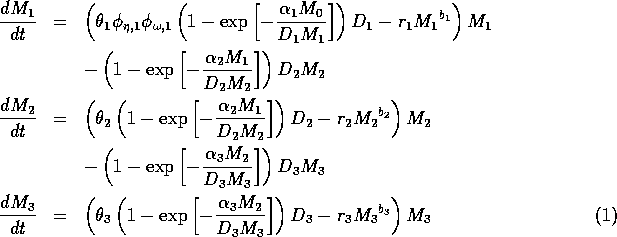
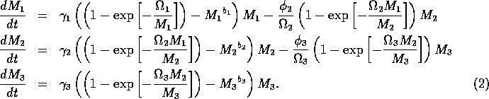
The model equations are functionally homogeneous (i.e., all three equations contain the same basic terms), because the authors argue that the same generalized functional and numerical responses must describe the search, acquisition, and conversion of all organisms as they seek to satisfy their metabolic requirements. Details of the model formulation can be found in Gutierrez et al. (1994). The final equations are:

  ,

where M₁ is the biomass of plants, M₂ is the biomass of herbivores, and M₃ is the biomass of predators. The parameters represent assimilation rates corrected for the efficiency of biomass conversion; represents the proportion of the resource that is available to its consumers (that is, its apparency); D_i is the per unit demand of the consumer for resources; r_i is the base respiration rate corrected for the efficiency of biomass conversion; and b_i is the degree of self-limitation. M₀ represents a biomass equivalent of the light energy incident in the growing space of the plants, and and (which both lie between 0 and 1) scale the potential photosynthesis rate to the realized rate.

The respiration term, r_iM_i^{1 + b_i}, requires further explanation. Respiration usually increases with population density (Gutierrez et al. 1994) and, thus, should be an increasing function of M_i. However, introducing such a functional dependence increases the model's complexity. Because the effect is usually small, the authors chose the simpler formulation r_iM_i^{1 + b_i}, where b_i has a value between 0.02 and 0.05. The disadvantage of this choice is that r_i must have rather unusual units (grams per b_i per day, where grams are the units of M_i) that depend on b_i. Thus, the term r_iM_i^{1 + b_i} has the same units as (namely, grams per day, where grams are the units of M_i). This dependence of the units on b_i is not satisfactory from a mathematical viewpoint, but since b_i is small, I chose to ignore this initially. In the next section, I discuss a small alteration to the model that takes care of the difficulty.

Gutierrez et al. (1994) use parameter values corresponding to a cassava (Manihotesculenta Crantz)-mealybug (Phenacoccuss manihoti Mat.-Ferr.)-parasitoid system in Africa. They claim that their analysis demonstrates that the parasitoid Epidinocarsis lopezi (De Santis) can control the mealybug (except on poor soils), whereas E. diversicornis (Howard) and native natural enemies cannot. However, the parameter values for the cassava-mealybug-parasitoid system given to me by the authors (only values for are reported in the paper) did not yield the isocline configurations or the behavior that they described. I then scaled the equations to get a better idea of the relative magnitudes of the parameters. The procedure involved is discussed in the next section.

A1.3 Nondimensionalization

The technique of nondimensionalizing, or scaling, is commonly used to simplify a system of equations because it has many other advantages. It illuminates which parameters are most important in determining the dynamics of the model (Edelstein-Keshet 1988) and gives insight into the relative magnitudes of the parameters required to produce biologically reasonable behavior. Also, the state variables are scaled so that they all have the same order of magnitude, say between 0 and 1. This is important when solving the equations numerically, as very different magnitudes can lead to computer round-off errors (Gerald and Wheatley 1989). In the cassava-mealybug-parasitoid system, the biomass of cassava is much larger than that of the mealybug and the parasitoid (cassava mass averages ~ 2 kg, whereas the mealybug and parasitoids have average masses of ~ 2 mg). Scaling, at least, is thus vital. (For an introduction to nondimensionalizing systems of ordinary differential equations, see Edelstein-Keshet 1988.)

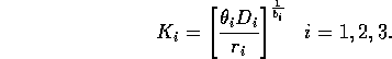
Natural scalings for the state variables are given by their carrying capacities when resources are abundant. Gutierrez et al. (1994) calculate these to be

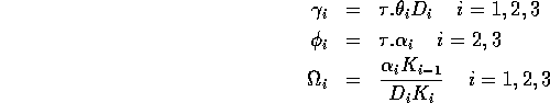
Replacing M_i by (i=1,2,3) , and t by (here K_i has the dimensions of M_i and the dimensions of t; hence, (i =1,2,3) and t* are dimensionless variables) and choosing the dimensionless combinations of parameters

,

where K₀ = M₀ gives the nondimensionalized Eqs. A1.2, where I have replaced by M_i and t* by t for convenience:

(I replaced the product by , because all three parameters have the same effect on the dynamics and, thus, do not need to be considered separately.)

The choice of dimensionless parameters is not unique. Other combinations would have led to slightly different final equations, but the choices here lend themselves to biological interpretation. For example, can be thought of as the potential per unit biomass growth rate (Gutierrez et al. 1994), or as the conversion efficiency of the consumer in converting the resource into biomass. can be thought of as the availability of the resource to the consumer, or perhaps the nutritional value of the resource. is made up of a ratio of quantities. The numerator can be thought of as the maximum amount of resource available to the consumer, and the denominator as the maximum demand of consumers for resource. More simply, gives a measure of the ratio of supply to demand. Results in Gutierrez et al. (1994) are based on the relationship between and , since is just a scaling factor. Hence, results using Eqs. A1.2 are comparable with those in Gutierrez et al. (1994).

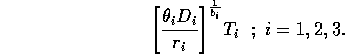
I mentioned earlier that the parameters r_i in the original model have units that depend on b_i. This can be prevented by replacing the terms r_iM_i^{1 + b_i} with terms of the form , where T_i has the same units as M_i. T_i can be thought of as a threshold value above which self-limitation becomes noticeable. With this modification, the units of r_i are per day, and r_i can be interpreted as a respiration rate, as was originally intended. The new carrying capacities are given by

It can be shown that setting the K_i 's equal to these new values and scaling the equations as above results in system (A1.2) once again. Thus, the problems with the respiration term can be ignored in the remainder of the paper.

Having scaled the equations, I needed to choose values for the parameters. An advantage of scaling is that there are now 11 parameters instead of the original 18. For comparison with the results of Gutierrez et al. (1994), I wanted to find values that resulted in isocline configurations similar to those in their paper. XPPAUT calculates and displays isoclines in two dimensions, and parameter values can be altered interactively. Since the competition effect is very small, but difficult to quantify, I followed A. Gutierrez (personal communication) and chose B_i = 0.02 (i = 1,2,3). Values of , , , , , , , gave the isocline configurations shown in Fig. 11 . These isoclines have similar shapes to those in Gutierrez et al. (1994). A noticeable difference is that the M₃ -isocline intersects the M₂ -isocline to the left of the M₂ -peak. In fact, using the techniques in Gutierrez et al. (1994), it would have been impossible to conclude that the tritrophic equilibrium is stable for the isocline configuration shown in Fig. 11, because of the position of the intersection point in the plane. For this parameter set (which I shall call the reference set), there is also a stable limit cycle. The initial values of M₁,M₂ and M₃ determine whether the system approaches the stable equilibrium or the limit cycle.

Biological considerations suggest that these values for the are rather high and that the value for is rather low. However, in the absence of better information and since this parameter set has a nontrivial, stable equilibrium point, it is a convenient starting point.

Before beginning an analysis of the model, I will introduce a small modification to the equations. Because the problems associated with ratio-dependent models described in section A1.1 involve low population densities, it would be interesting to know what effects a small modification to the model, which prevents the denominators of the ratios from getting too close to zero, would have on the dynamics. Abrams (1994) states that modifications to ratio-dependent models cannot be made biologically realistic because the original models have no clear mechanistic derivation. However, some form of modification that prevents the ratios from tending to infinity may be useful for revealing any spurious behavior near the axes that may result from the ratio dependence.

The ratios in model (A1.2) have the form

.

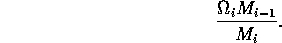The difficulties are experienced when M_i approaches zero. Adding a constant in the denominator, that is, replacing the ratio by

would alleviate the problem. Although this addition may appear difficult to justify biologically, Gutierrez (1992) used an exponent of this form in his functional response term. That model is physiologically based, as is the present one.

In model A.1.2 ], the ratio-dependent terms have the form

  ,

where k is a parameter or combination of parameters. When the exponent is small, we have

.

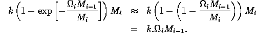In order to preserve this property when using the modified term (Eq. A1.3 ), I replaced Eq. A1.4 by

,

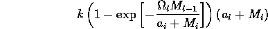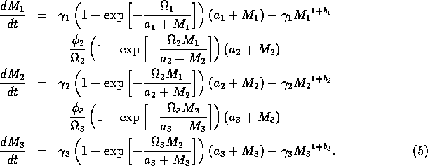
where a_i is a small constant, say 0.001. The resulting equations are:

  .

If a_i = 0 (i = 1, 2, 3) , then the above model is equivalent to system (A1.2).